PAST - Case study 3 - Morphometrics of Ordovician trilobites

Case study 3 - Morphometrics of Ordovician trilobites

Data files: glaber.dat, linnars1.dat og linnars2.dat

Norwegian illaenid trilobite (Paleontological Museum, Oslo). Length approx. 6 cm.

Although distinctive and often common in Ordovician faunas, illaenid trilobites have relatively featureless, smooth exoskeletons; taxonomic discrimination within the group is therefore difficult. While a number of authors have attempted a qualitative approach to illaenid systematics, Bruton & Owen (1988) described the Norwegian Upper Ordovician members of the family in terms of measurements and statistics. This study seeks to discriminate between at least two different species of the illaenid trilobite Stenopareia.

Four measurements made on the cranidia of the Norwegian illaenid trilobites are defined on the figure. L2, W1, W2 and W3 have been measured on Stenopareia glaber from the Ashgill of Norway (glaber.dat) together with S. linnarssoni from both Norway (linnars1.dat) and Sweden (linnars2.dat). A previous study of S. glaber recognized long and short forms. The first specimen recorded in glaber.dat is a typical long form, the second a typical short form and the third, the lectotype of S. glaber. The remaining measurements relate to further specimens of S. glaber.

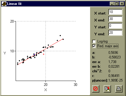
Open glaber.dat, and 'commatize' if necessary. Using 'Row color/symbol' in the Edit menu, assign the symbol '+' to row 1 (typical long form), square to row 2 (typical short) and 'x' to row 3 (lectotype). Select the L2 and W1 columns, and choose 'Linear' in the Model menu:

Repeat the exercise with different pairs of variates (L2/W1/W2/W3) plotted against each other. You may have to move columns by dragging the column labels. How do the typical long, short and lectotypic individuals relate to the sample as a whole? Is there any justification for splitting the sample into long and short forms?

Graphical comparison of data sets

We now want to include all three data files in the analysis. Open glaber.dat again. Click in the cell at row 44, column L2. Choose 'Insert file' in the File menu, and insert the file linnars1.dat. Assign the symbol '+' (red) to the newly inserted rows. Click in the cell at row 54, column L2. Choose 'Insert file' in the File menu, and insert the file linnars2.dat. Assign the square symbol (blue) to the newly inserted rows. If you want, you can save the concatenated data set as Illaenid.dat.

Repeat the plotting procedure above (linear fit) for the concatenated data set. For the variety of measurements available, is there a partition between samples on any of the possible XY plots?

Principal Components Analysis

Select the whole matrix, and choose 'Principal components' in the Multivar menu. Use the 'Var-covar' option. How much of the variance in the data set is accounted for by the first component? Select 'View loadings' in the Principal Components window:

All four variables have relatively similar, positive loadings on the first component. Can you interpret this first component in morphological terms? Also look at the loadings for component 2 and 3, and interpret these.

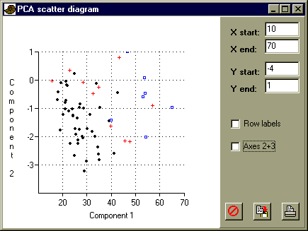
Now choose 'View scatter' in the Principal Components window to see the specimen scores on the two first components:

Are the groups well separated? Tick the 'Row labels' box to identify specimen 1 (long form) and 2 (short form) in the S. glaber group. Does their placement on the diagram correspond with your interpretation of component 2?

More information about Principal Components analysis can be found in the manual.

Principal Coordinates Analysis

Select the whole matrix, and choose 'Principal coordinates' in the Multivar menu. Are the groups well separated along the arch?

Cluster Analysis

Select the whole matrix, and choose 'Cluster analysis' in the Multivar menu. Use the Euclidean similarity measure. Do the clusters correspond with the two proposed species? Which morphological parameter do you think is primarly responsible for the clustering pattern?

Discriminant analysis

Next, tag all the S. linnarssoni rows with red, select all, and choose 'Discriminant' in the Multivar menu. Set the bin start value to -30 in order to see the whole histogram. Are the S. glaber and S. linnarssoni data points well separated? Again, which morphological parameter is probably responsible for most of the spread along the discriminant axis?

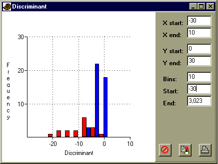
More information about discriminant analysis can be found in the manual.

Conclusion

Bruton & Owen (1988) recognised two species, S. glaber and S. linnarssoni, in their detailed study. Does your analysis support their findings?