Discussion

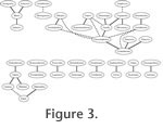
To complete our analysis we briefly discuss some of the correlations produced with the methods described in this paper and their ecological interpretation. We look at two sets of correlations that both are produced using criteria Time and NoTaxonomic, but with different geographic base sets. In Figure 2 we show all significant positive and negative correlations when looking only at the union of the areas covered by the two species (GeoUnion), and in Figure 3 all significant positive and negative correlations between the species without using a geographic filtering criteria (NoGeo). In the figures, species are presented as ellipses, positive correlations as bold lines, and negative correlations as dashed lines.

The correlation patterns observed are clearly very sensitive to geographic restrictions. The geographically restricted set in Figure 2 shows mostly correlations that can be plausibly explained by ecology. Thus, Stephanorhinus and Cervus are two of the main genera of interglacial (warm) assemblages of the Pleistocene Ice Age, while Mammuthus and Equus characterise the glacial (cold) assemblages that alternate with the interglacial ones. The biogeography of these assemblages was dynamic (Koenigswald 2007), with alternating expansion from refugia, so the correlations are not likely to be driven by geography. Among the geologically older genera the cluster around Gazella is made up of other open-adapted taxa (Palaeotragus, Tragoportax, Microstonyx), with negative correlations to forest taxa (Euprox, and indirectly Propotamochoerus and Amphicyon). The genera negatively correlated to the open-adapted Ceratotherium and Choerolophodon are also primarily forest taxa (Dihoplus, Aceratherium, Tetralophodon and, with some reservations, Deinotherium). The carnivore cluster around Martes also represents a forest setting.

As expected, the correlations in the geographically unrestricted case in Figure 3 appear in many cases to be due primarily to distribution patterns. The cluster around Tapirus as well as several pairs of genera belong to this group, for example Pleasiaceratherium-Prosanthorhinus, Procervulus-Lagomeryx, Helladotherium-Pachytragus, and Pseudotragus-Criotherium. Among negatively correlated pairs, Euprox-Gazella and Euprox-Choerolophodon belong to this category. The main reason for these geographic associations is, however, not so much random spatial patterns as a strong underlying and ultimately climatological forcing: the distribution of the genera reflects the distribution of the ecological associations ("chronofaunas") to which they belong (Eronen et al. 2009), essentially the forested western and central European faunas versus the open woodlands of eastern Europe and western Asia (Fortelius et al. 1996).

Some pairs in the geographically unrestricted set appear to be related to other factors than geography. The negative correlation of Anchitherium-Miotragocerus is likely caused by nearly non-overlapping temporal distributions. Two pairs of widely distributed carnivores are unlikely to be explained by geographic distribution, unless by chance, but appear instead to be related through foraging behaviour to habitat: Vulpes (red fox) and Nyctereutes (raccoon dog) are both short-legged generalists strongly associated with vegetation cover, while Acinonyx (cheetah) and Chasmaporthetes (cheetah-like hyaena) represent extremely long-legged pursuit predators in open habitats.

When looking at the data in Figure 2 and Figure 3, it is important to keep in mind that it reports results that are statistically significant, but the absence of a correlation is not significant. Our statistical methodology allows us to report results that are backed up by data, but in interpretation the absence of a correlation should not be considered as a significant result. Absence of a correlation means that there is not enough evidence for the correlation in the data, but it does not mean that the two species must be non-related. Correlations are also not transitive: significant correlations of A and B, and of B and C, do not necessarily imply a significant correlation of A and C.