RESULTS
 The entire data set including both previously published and new samples are in
Appendix 1 and 2. The entire data set including both previously published and new samples are in
Appendix 1 and 2.
Species Diversity
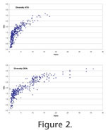
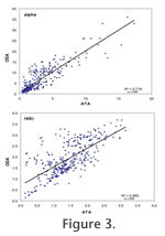
Plots of Fisher alpha against H(S) are similar for ATAs and ODAs although the range is somewhat extended for the latter (Figure 2). There is a significant positive linear correlation between the ATAs and ODAs for both diversity indices but the correlation is stronger for Fisher alpha (R2 = 0.778) than for the information function (R2 = 0.485,
Figure 3).
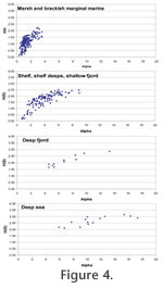
 There is a progression from low diversity in marsh and marginal marine, through shelf seas, shallow fjord, shelf deeps and Skagerrak, deep fjord >500 m and deep sea (Figure 4). See
Table 2 for the distribution of diversity values for each environment together with the mean and standard deviation. Overall, there is an increase in diversity with water depth: deeper than 500 m alpha is >5. Deeper than100 m H(S) rarely goes below 1.0. There is a progression from low diversity in marsh and marginal marine, through shelf seas, shallow fjord, shelf deeps and Skagerrak, deep fjord >500 m and deep sea (Figure 4). See
Table 2 for the distribution of diversity values for each environment together with the mean and standard deviation. Overall, there is an increase in diversity with water depth: deeper than 500 m alpha is >5. Deeper than100 m H(S) rarely goes below 1.0.
Non-metric Multi-dimensional Scaling (MDS)
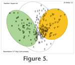
Samples that plot close together have similar faunal composition; those that plot far apart are different.
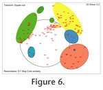
 Because the faunas of marginal marine marshes and estuaries are fundamentally distinct from those of the shelves, we have presented MDS of these data as separate plots (Figure 5,
Figure 6). Because the faunas of marginal marine marshes and estuaries are fundamentally distinct from those of the shelves, we have presented MDS of these data as separate plots (Figure 5,
Figure 6).
Marsh and estuary. When individual geographic areas are plotted separately there is varying degree of overlap (indicating local differences) of the estuaries (Exe, Christchurch, Poole, Hamble in England; shallow waters around Oslofjord, Kattegat and Skagerrak in Norway, Denmark and Sweden) and relatively little overlap with the field for marshes. The overall picture becomes even clearer when the data are plotted as marsh (M), estuary <3 m deep (E) and >3m deep (E*) (Figure 5). This is a reflection of the fact that many of the marsh taxa are confined to marsh habitats.
 Shelf seas to deep sea (Figure 6). Overall, the ATA faunal composition of the main study areas are reasonably distinct although there is some overlap with the Channel/Celtic Sea (CC), the southern North Sea (NS) and the Scottish shelf deeps (MD). The Skagerrak field (SK) includes outer Oslofjord (OF) and outer Lyngdalsfjord (YL). Loch Etive (Et) is more closely similar to the UK shelf seas than the deep Hardangerfjord (H). The latter lies between SK and the deep sea (NE) with one sample overlapping the latter. Shelf seas to deep sea (Figure 6). Overall, the ATA faunal composition of the main study areas are reasonably distinct although there is some overlap with the Channel/Celtic Sea (CC), the southern North Sea (NS) and the Scottish shelf deeps (MD). The Skagerrak field (SK) includes outer Oslofjord (OF) and outer Lyngdalsfjord (YL). Loch Etive (Et) is more closely similar to the UK shelf seas than the deep Hardangerfjord (H). The latter lies between SK and the deep sea (NE) with one sample overlapping the latter.
Depth Distributions of Species
 Because our data set extends from intertidal to deep sea (4250 m) we have been able to determine the depth distributions of species (ranges) within those extremes. These are summarised in
Table 3. There is a progressive change in faunal composition with increasing depth but there are no obvious depth-related boundaries. However, there are some differences in relative abundance in the various environments. Because our data set extends from intertidal to deep sea (4250 m) we have been able to determine the depth distributions of species (ranges) within those extremes. These are summarised in
Table 3. There is a progressive change in faunal composition with increasing depth but there are no obvious depth-related boundaries. However, there are some differences in relative abundance in the various environments.
 For instance, Adercotryma wrighti reaches abundances of nearly 60% on shelf seas at depths of 100-130 m whereas in Hardangerfjord and the deep sea it never exceeds 16%. For instance, Adercotryma wrighti reaches abundances of nearly 60% on shelf seas at depths of 100-130 m whereas in Hardangerfjord and the deep sea it never exceeds 16%.
Distribution by Environment and Geography
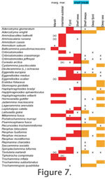
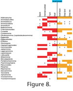 The distribution patterns are presented by environment (Figure 7, species;
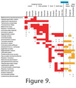
Figure 8, genera) and by geography (Figure 9). The shallow water areas (<6 m) around Oslofjord, Skagerrak and Kattegat are treated as marginal marine (estuarine) here as they are brackish. The distribution patterns are presented by environment (Figure 7, species;
Figure 8, genera) and by geography (Figure 9). The shallow water areas (<6 m) around Oslofjord, Skagerrak and Kattegat are treated as marginal marine (estuarine) here as they are brackish.
There is a clear progression of species from marsh to deep sea (Figure 7.2). Typical marsh species such as Jadammina macrescens and Trochammina inflata also occur in adjacent non-vegetated intertidal flats. Likewise, some intertidal taxa are present in low abundance on marshes. The faunas of shelf seas, shelf deeps and shallow fjord (Etive) have much in common.
 Those of the deep Hardangerfjord overlap the shelf seas and deep seas. The pattern for genera is somewhat different (Figure
8) because some span a broad spectrum of environments (e.g., Haplophragmoides, Reophax, Cribrostomoides, Adercotryma, Eggerelloides, Portatrochammina). Superimposed on the environmental controls on distribution there is also a geographical component. Although most species are found throughout the geographic range of their environment (Figure 9) some are more restricted. For instance, the marsh species Tiphotrocha comprimata is confined to Norway and Balticammina pseudomacrescens has yet to be found in the marshes of Sweden and Denmark. Ammotium cassis is absent from Britain. Liebusella goesi is rare in shelf seas and most abundant in deeper water (Norwegian fjords, Skagerrak and shelf deeps off Scotland) but not on the continental slope. Those of the deep Hardangerfjord overlap the shelf seas and deep seas. The pattern for genera is somewhat different (Figure
8) because some span a broad spectrum of environments (e.g., Haplophragmoides, Reophax, Cribrostomoides, Adercotryma, Eggerelloides, Portatrochammina). Superimposed on the environmental controls on distribution there is also a geographical component. Although most species are found throughout the geographic range of their environment (Figure 9) some are more restricted. For instance, the marsh species Tiphotrocha comprimata is confined to Norway and Balticammina pseudomacrescens has yet to be found in the marshes of Sweden and Denmark. Ammotium cassis is absent from Britain. Liebusella goesi is rare in shelf seas and most abundant in deeper water (Norwegian fjords, Skagerrak and shelf deeps off Scotland) but not on the continental slope.
 Controls on Distribution Patterns Controls on Distribution Patterns
As many data as possible have been gathered on environmental parameters. This includes our own measurements made at the time of sampling and data from the literature (Appendix 1 and 2). Unfortunately, there is not a complete environmental data set for every sample.
 Data on maximum bottom water temperatures are more complete than those on minimum values and this is true also for salinity. As noted above, the sea floor organic flux is calculated from satellite imagery in those areas away from the coast where suspended sediment is minimal or absent. Nevertheless, some useful conclusions can be drawn about the relationships between environmental parameters and the foraminiferal assemblages. Data on maximum bottom water temperatures are more complete than those on minimum values and this is true also for salinity. As noted above, the sea floor organic flux is calculated from satellite imagery in those areas away from the coast where suspended sediment is minimal or absent. Nevertheless, some useful conclusions can be drawn about the relationships between environmental parameters and the foraminiferal assemblages.
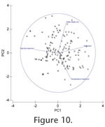
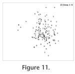
Principal component analysis and MDS plots of marsh and shallow water environments (Appendix 1, marginal marine;
Figure 10 and Figure 11) show a large scatter of points with marsh samples occupying a distinct field which slightly overlaps that of the rest of the samples and which seems primarily determined by water depth. Otherwise, there are no clear correlations between different geographic areas and the environmental variables.
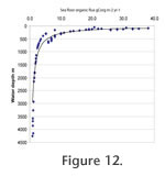 For shelf seas, down to about 300 m, the Corg shows a wide range of 8-38 g Corg m-2 yr-1 which narrows to 6-23 and 2.7-5.2, respectively, for shelf deeps and deep fjord, and to 0.9-2.1 g Corg m-2 yr-1 in the deep sea (Figure 12). For shelf seas, down to about 300 m, the Corg shows a wide range of 8-38 g Corg m-2 yr-1 which narrows to 6-23 and 2.7-5.2, respectively, for shelf deeps and deep fjord, and to 0.9-2.1 g Corg m-2 yr-1 in the deep sea (Figure 12).
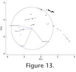 There is a positive linear correlation between water depth and maximum temperature (R2 = 0.5051) and hence between sea floor organic flux and maximum temperature (R2 = 0.5819), and a weak positive correlation between sea floor organic flux and sediment grain size (R2 = 0.2953). Multivariate analysis of the abiotic factors plus sea floor organic flux shows a clear pattern (Figure 13). The vectors for the environmental parameters on the PCA plot show that the primary control on the deep sea (D), Skagerrak (SK) and Hardangerfjord (H) is a combination of water depth and maximum temperature. These areas are also separated from one another by sediment grain size differences. The shelf sea environments are separated primarily on their sediment characteristics and to a lesser extent on sea floor organic flux (finer sediment and lower sea floor organic flux in the Forties (F) and Ekofisk (Ek) areas of the North Sea than in the Celtic Sea (C)). There is a positive linear correlation between water depth and maximum temperature (R2 = 0.5051) and hence between sea floor organic flux and maximum temperature (R2 = 0.5819), and a weak positive correlation between sea floor organic flux and sediment grain size (R2 = 0.2953). Multivariate analysis of the abiotic factors plus sea floor organic flux shows a clear pattern (Figure 13). The vectors for the environmental parameters on the PCA plot show that the primary control on the deep sea (D), Skagerrak (SK) and Hardangerfjord (H) is a combination of water depth and maximum temperature. These areas are also separated from one another by sediment grain size differences. The shelf sea environments are separated primarily on their sediment characteristics and to a lesser extent on sea floor organic flux (finer sediment and lower sea floor organic flux in the Forties (F) and Ekofisk (Ek) areas of the North Sea than in the Celtic Sea (C)).
|