FIGURE 1. Scheme depicting the measured parts of antenna (ant) and mandible (md): d1 = diameter of the mandibular exopod (ex); d2 = diameter of the antennal exopod; d3 = diameter of the antennal endopod (en); h = height of the antennal coxa (cx) in proximal-distal axis; l = length of the antennal coxa in median-lateral axis. Other abbreviation: bas = basipod.
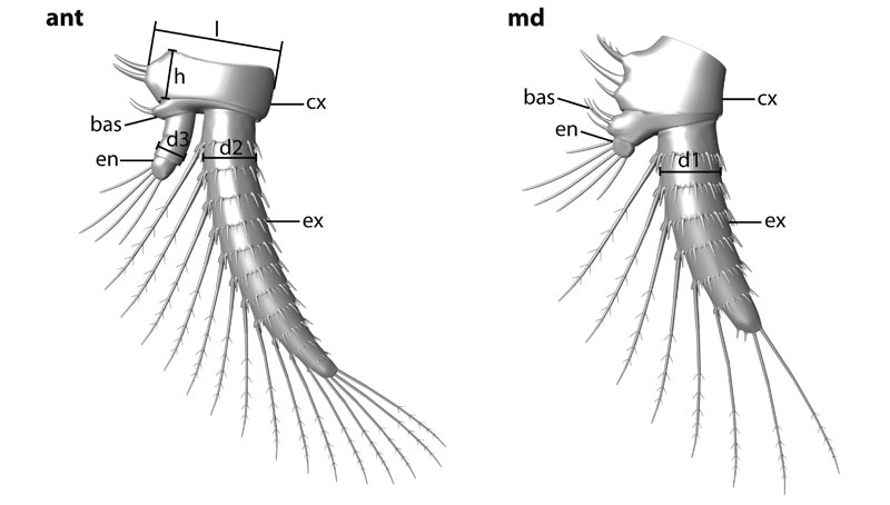
FIGURE 2. Scatter and box plots of the measured parameters. 2.1. Diameter of the mandibular exopod (d1) versus diameter of the antennal exopod (d2). 2.2. Diameter of the antennal endopod (d3) versus diameter of the antennal exopod (d2). 2.3. Height of the antennal coxa in proximal-distal axis (h) versus length of the antennal coxa in median-lateral axis (l). 2.4. Diameter of the antennal exopod (d2) versus length of the antennal coxa in median-lateral axis (l). 2.5. 3D scatter plot of specimens of which d2, d3 and l could be measured. 2.6. Box plot of parameter d2; three size classes highly significant (Wilks Lambda = 0.097, F = 12.505, p < 0.0001).
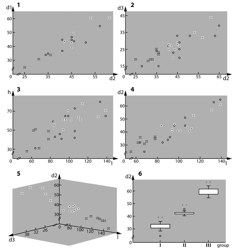
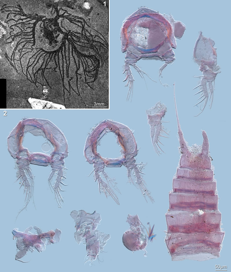
FIGURE 3. Red-blue stereo images of very well preserved specimens processed after the method of Haug J.T. et al. (2009b). 3.1. Best preserved specimens of size class III (top; collection number AUGD 12449B [AUGD omitted in the following]), II (middle; 12448A), and I (bottom; 12449E) respectively; all three specimens to the same scale. 3.2. 12449C. 3.3. 12449A02. 3.4. 12449A10. 3.5. 12449A04. Abbreviations: atl = antennula; cs = cephalic shield; la = labrum; sl = setule; sp = spine; ss = surrounding seta; st = seta. Other abbreviations as before.
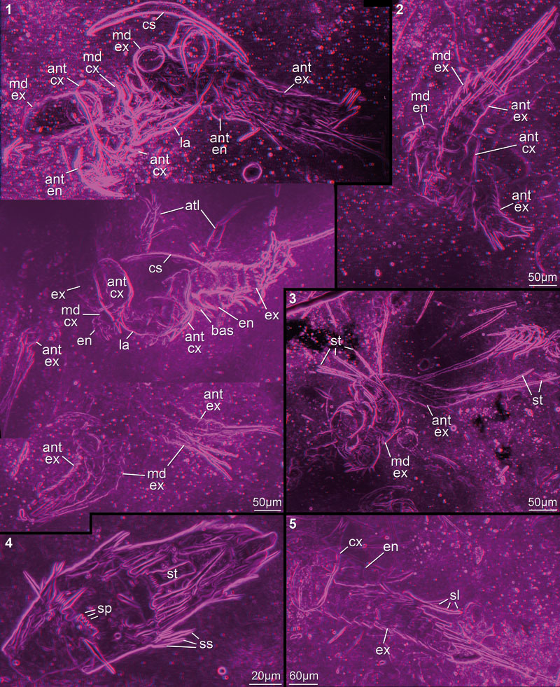
FIGURE 4. Red-blue stereo images of well preserved specimens processed after the method of Haug J.T. et al. (2009b). This method is disadvantageous here, as strongly contrasted areas of the matrix, so-called "curtains" (ct), appear to cut the animal into two halves. 4.1. 12449A25. 4.2. 12449A05. 4.3. 12449A08.
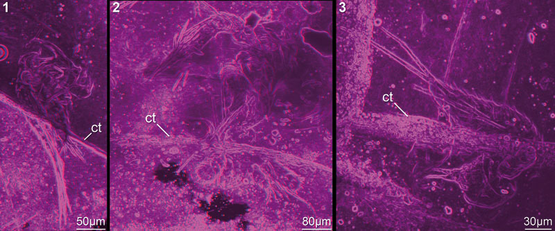
FIGURE 5. Red-blue stereo images of very well preserved specimens. 5.1–2. Rather complete specimens indicating position of appendages in relation to each other. 5.1. 12449B. 5.2. 12448A. 5.3–5. Mandible with many details preserved; 12449A01. 5.3. Entire specimen. 5.4. Terminal setae with setules and visible subdivision (arrow). 5.5. Spines on basipod and coxa. Abbreviations as before.
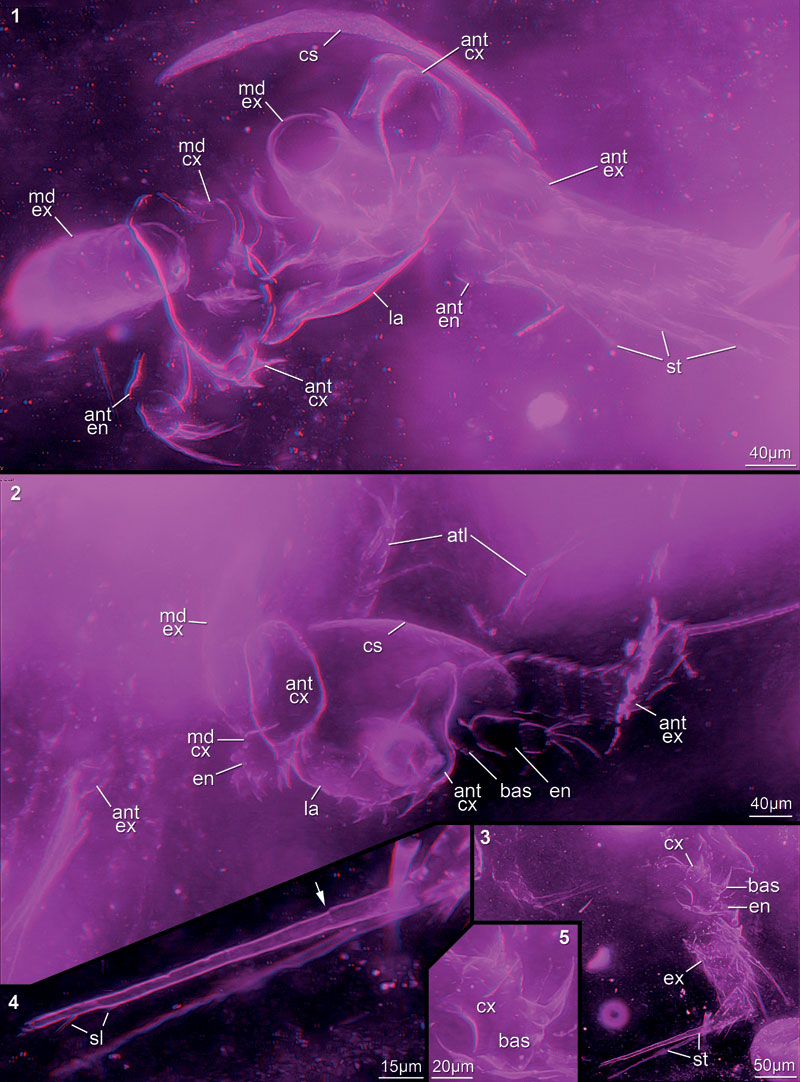
FIGURE 6. Red-blue stereo images of well preserved specimens mainly representing several appendages of one nauplius. 6.1. 12448B. 6.2. 12449C. 6.3. 12449A25. 6.4. 12449A02. 6.5. 12449A03. 6.6. 12449E. 6.7–8. 12449A04. 6.8. Minute setules preserved. Abbreviations as before.
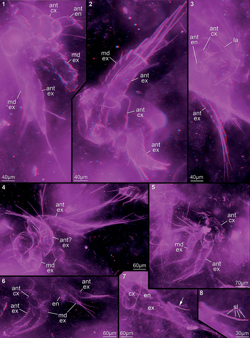
FIGURE 7. Red-blue stereo images of well preserved specimens, but in cloudy-appearing matrix. 7.1. 12445D. 7.2. 12449A20. 7.3. 12449A18. 7.4. 12451F. 7.5. 12447C. 7.6. 12447A. 7.7. 12449A22. Abbreviations as before.
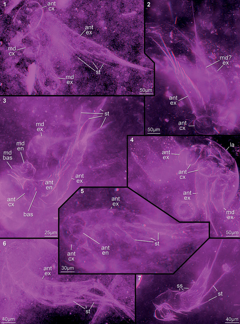
FIGURE 8. Red-blue stereo images of well preserved specimens, but matrix contains many particles or "curtains" (supposedly cracks). 8.1. 12449A05. 8.2. 12449A06. 8.3. 12449A08. 8.4. 12449A16. 8.5. 12449A09. 8.6. 12449A14. 8.7. 12449A19. 8.8. 12447B. 8.9. 12454C. Abbreviations as before.
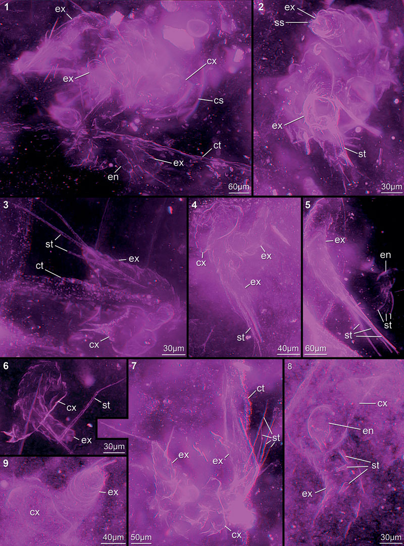
FIGURE 9. Red-blue stereo images of appendage fragments, mainly parts of exopods (9.1–8), but also coxae (9.9–11). 9.1. 12452B. 9.2. 12449A21. 9.3. 12449A10. 9.4. 12451B. 9.5. 12447F. 9.6. 12449G. 9.7. 12454F. 9.8. 12442E. 9.9. 12454D; supposed coxa in unusual preservation. 9.10. 12451C. 9.11. 12449A15. Abbreviations as before.
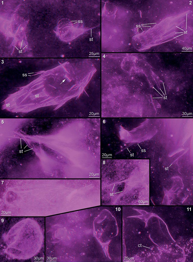
FIGURE 10. Red-blue stereo images of appendage fragments in cloudy-appearing matrix areas, probably all representing exopod fragments. 10.1. 12442B. 10.2. 12445A. 10.3. 12447E. 10.4. 12447D. 10.5. 12444B. 10.6. 12448E. 10.7. 12448F. 10.8. 12449A23. 10.9. 12454G. 10.10. 12454I. 10.11. 12454B. 10.12. 12454H. 10.13. 12451D. Abbreviations as before.
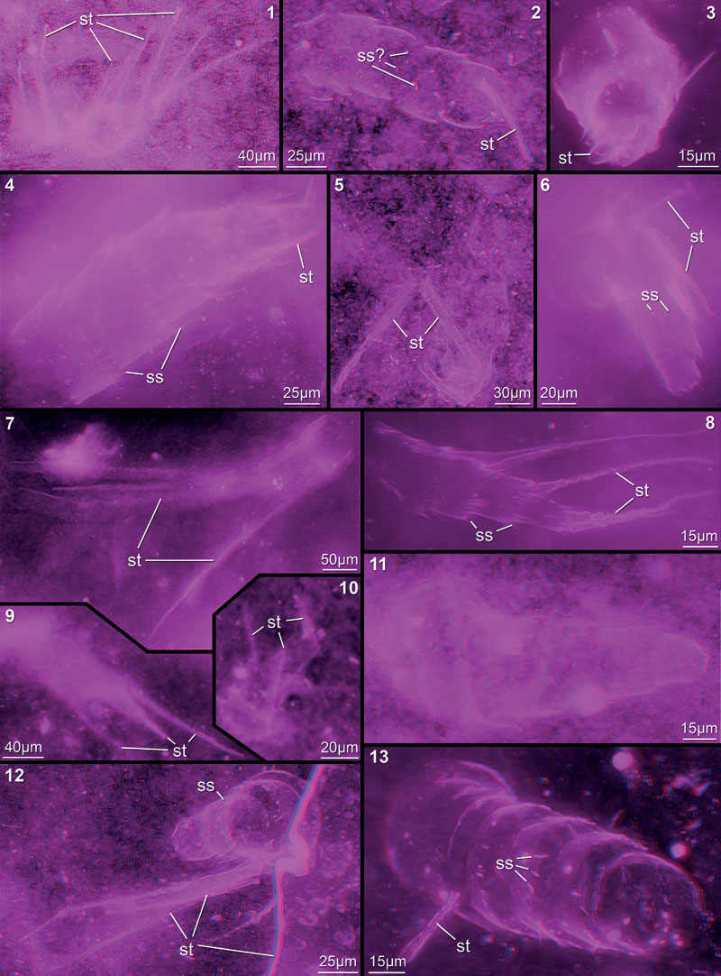
FIGURE 11. Red-blue stereo images of rather faintly preserved specimens, but still several details visible. 11.1. 12454E. 11.2. 12442D. 11.3. 12448G. 11.4. 12454A. 11.5. 12451A. 11.6. 12445F. 11.7. 12449A17. 11.8. 12449A11. 11.9. 12449A07. Abbreviations as before.
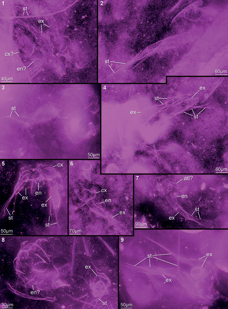
FIGURE 12. Red-blue stereo images of faintly preserved specimens; still assignment to here presented nauplius larvae possible due to preserved details. 12.1. 12451G. 12.2. 12449D. 12.3. 12449A13. 12.4. 12448C. 12.5. 12449F. 12.6. 12449A12. 12.7. 12452A. 12.8. 12449A24. 12.9. 12451E. Abbreviations as before.
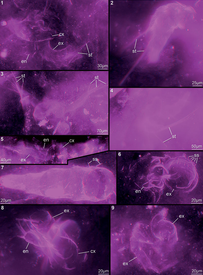
FIGURE 13. Red-blue stereo images of faintly preserved specimens in cloudy-appearing or particle-contaminated matrix areas. 13.1. 12442A. 13.2. 12444A. 13.3. 12442C. 13.4. 12448D. 13.5. 12445E. 13.6. 12448H. 13.7. 12445B. 13.8. 12447G. 13.9. 12442F. Abbreviations as before.
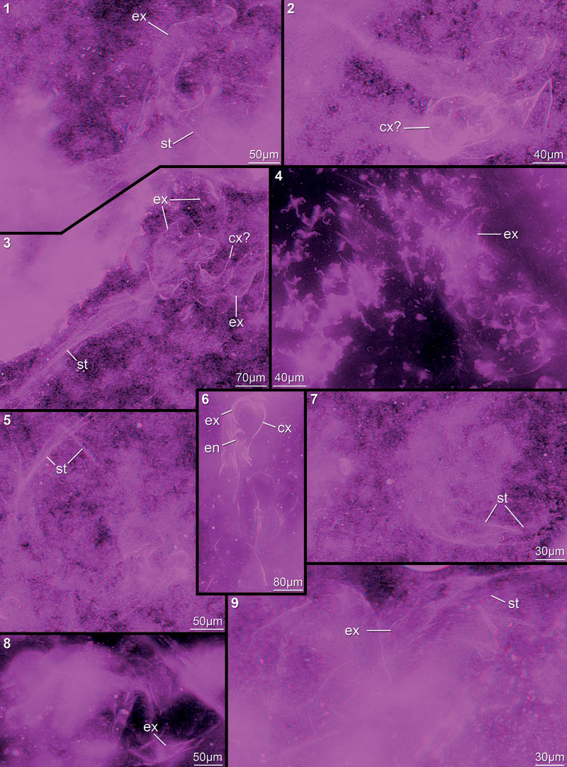
FIGURE 14. Red-cyan stereo image of 3D reconstruction of the here described nauplius in ventral view. Body in dark grey to indicate lacking data.
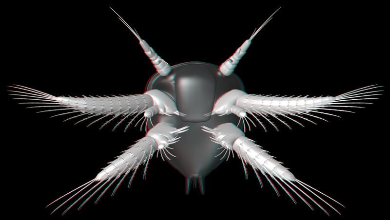
FIGURE 15. Fossil material for comparisons. 15.1. Marria walcotti Ruedemann, 1931 (USNM 83485A), a graptolite colony formerly erroneously interpreted as a crustacean nauplius; photographed under polarised light. 15.2. Dissected Holocene representative of the copepod species Enhydrosoma gariensis Gurney, 1930 (NHM In 51842); documented under transmitted light microscope with differential interference contrast (DIC).