Figure 1. A virtual peel, i.e., an inverted red-cyan stereo image, of the new specimen of Ursquilla yehoachi (Remy and Avnimelech, 1955), SMNS 67703. The specimen represents the posterior part of the body, including the telson and the three posterior pleomeres. Use red-cyan stereo glasses to view. Abbreviations: bs? = possible basipodal spine; dex = distal part of exopod; plm = pleomere; tel = telson; tpl = tergopleura; urp en = uropodal endopod; urp ex = uropodal exopod.
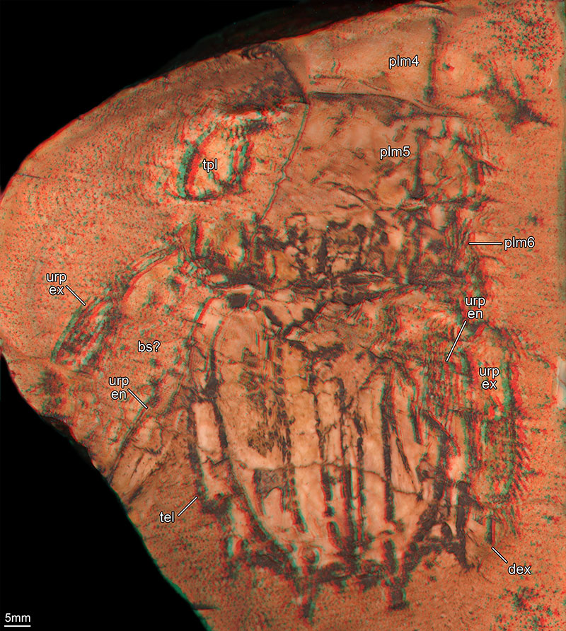
Figure 2. Details of the new specimen of Ursquilla yehoachi (Remy and Avnimelech, 1955), SMNS 67703. 2.1–2. Composite autofluorescence images (e.g., Haug, J.T. et al., 2008). Note that under fluorescence settings there are details visible, e.g., exact shape of the spines on the uropodal exopod, which are not visible under white-light conditions (see Figures 1, 2.3). 2.1. Part of the possible endopod of the left uropod and left part of the telson. 2.2. Right uropod with the articulated distal part of the exopod. 2.3. Virtual peel of the same area as in Figure 2.2. Use red-cyan stereo glasses to view. Abbreviations as before.
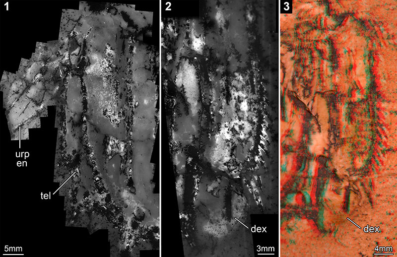
Figure 3. Red-cyan stereo images of all other known specimens of Ursquilla yehoachi (Remy and Avnimelech, 1955). 3.1, 3.2 and 3.4 are virtual peels, 3.3 is a normal stereo image. Use red-cyan stereo glasses to view. 3.1. Two specimens on one slab, BMNH I 7316, collections of the Natural History Museum London. 3.2. Specimen from the collections of the Geological Survey of Israel, Jerusalem, GSI M-8113. 3.3. Resin cast of the holotype (see Figure 3.4), BMNH I 15472, collections of the Natural History Museum London. 3.4. Holotype, MNHN R. 62691, from the collections of the Muséum national d'Histoire naturelle Paris.
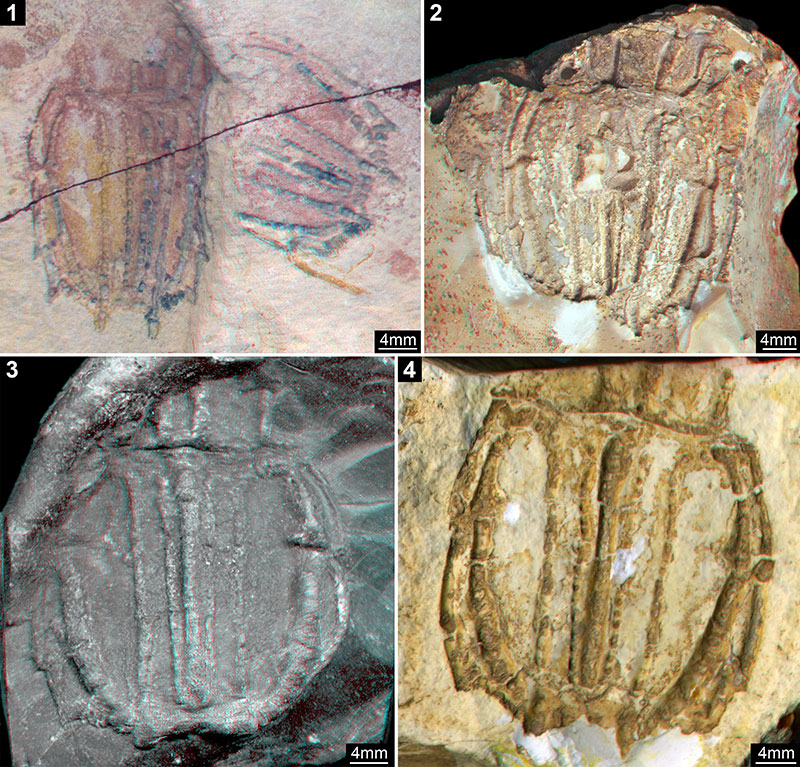
Figure 4. Method comparison and comparison with an extant specimen. All images are red-cyan stereo images, use red-cyan stereo glasses to view. 4.1–3. Specimen SMNS 67703 of Ursquilla yehoachi (Remy and Avnimelech, 1955). 4.1–2. Virtual surface models. 4.1. Surface model based on a micro-CT scan. 4.2. Surface model based on a surface scan of a peel out of dental casting compound of the fossil. 4.3. Virtual peel (same as Figure 1) for comparison. 4.4. The posterior region of an air-dried specimen of Squilla mantis (Linnaeus, 1758) for comparison, processed as the specimen in Figure 3.3, i.e., without depth inversion (normal stereo image). Images not to scale.
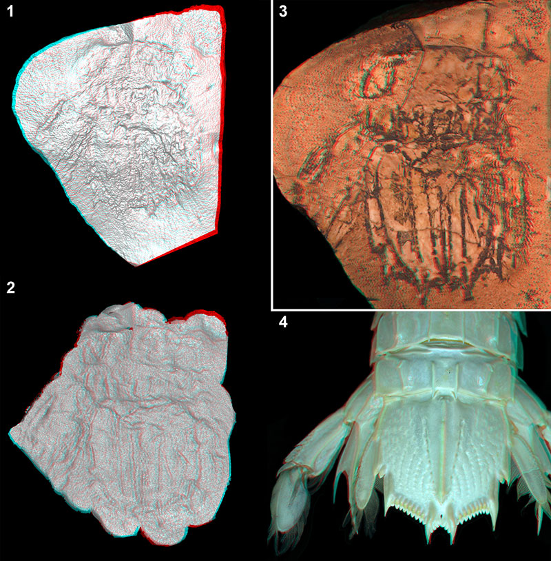
Figure 5. Tentative reconstruction of Ursquilla yehoachi (Remy and Avnimelech, 1955), represented as a scientific pencil drawing.
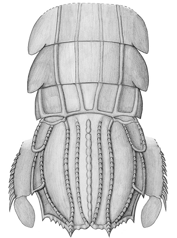
Figure 6. Uropod exopods of different Mesozoic and extant stomatopods and their phylogenetic positions within Unipeltata s. l. Arrow marks the occurrence of a bipartite uropodal exopod. 6.1. Sculda pennata Münster, 1840. 6.2. Pseudosculda laevis (Schlüter, 1874). 6.3. Supposed pseudosculdid from the Cretaceous of Mexico (Vega et al., 2007). 6.4. The herein re-evaluated Ursquilla yehoachi (Remy and Avnimelech, 1955); reconstruction, based on the new data. 6.5. Squilla mantis (Linnaeus, 1758). See Haug, J.T. et al. (2010) for details on relationships within Stomatopoda.
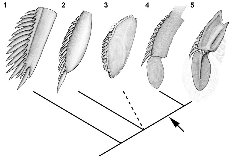
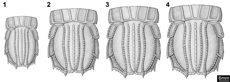
Figure 7. Size comparison of the known specimens of Ursquilla yehoachi (Remy and Avnimelech, 1955). To compare the length-to-width ratios, the reconstruction of the new specimen (SMNS 67703) was deformed according to the measured sizes of each of the other specimens. Lengths and widths given according to the illustrated part. 7.1. BMNH I 7316 (both specimens on this slab are of the same size; length: 3.1 cm, width: 1.9 cm, ratio: 1.6). 7.2. SMNS 67703 (length: 4.0 cm, width: 3.0 cm, ratio: 1.3). 7.3. GSI M-8113 (length: 4.2 cm, width: 3.2 cm, ratio: 1.3). 7.4. MNHN R. 62691 (Holotype) (length: 4.4 cm, width: 3.3 cm, ratio: 1.3).