FIGURE 1. Animation of 3-D reconstruction of a crinoid holdfast from CT z-sections. Eucalyptocrinites crassus Waldron, Indiana. Field Museum P569. Click on image to activate.
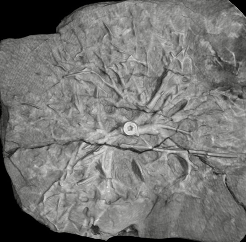
FIGURE 2. 1. The original image of the crinoid specimen (Eucalyptocrinites crassus, Silurian, Waldron Shale, Waldron, IN. USNM S 366). The black and white scale bar equals 1 cm. 2. Image subset or tile used in the demonstrations throughout this paper. The tile is 512 pixels by 512 pixels. 3. The steps of digital extraction through image segmentation. All photos underwent pre-processing, processing, and post-processing. However, the actual techniques used for each step varied and, in some cases, multiple steps were used. For example, for many of the images both CC analysis (CCA) and binary image morphology were used to improve the quality of the thresholding. A photo of a crinoid root segment is used in here to provide examples of the products of each step.
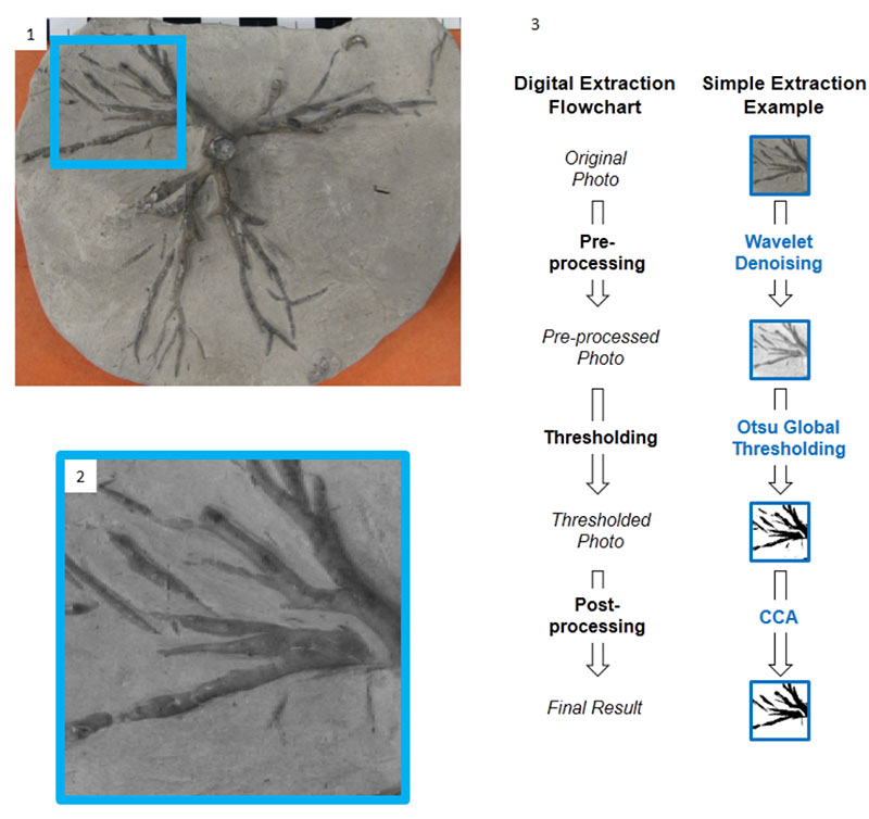
FIGURE 3. Left column: original images of crinoid holdfast. On the right: cleanly segmented images produced from images in the left column by combining several traditional and computer techniques. These segmented images can be used in morphometrics. 1. USNM S366. Frank Springer collection, Waldron, Indiana. 2. Field Museum, U.C. 56306, Waldron, Indiana. 3. USNM 42233, Ulrich collection, Waldron, Indiana. 4. USNM 42233, Ulrich collection, Waldron, Indiana.
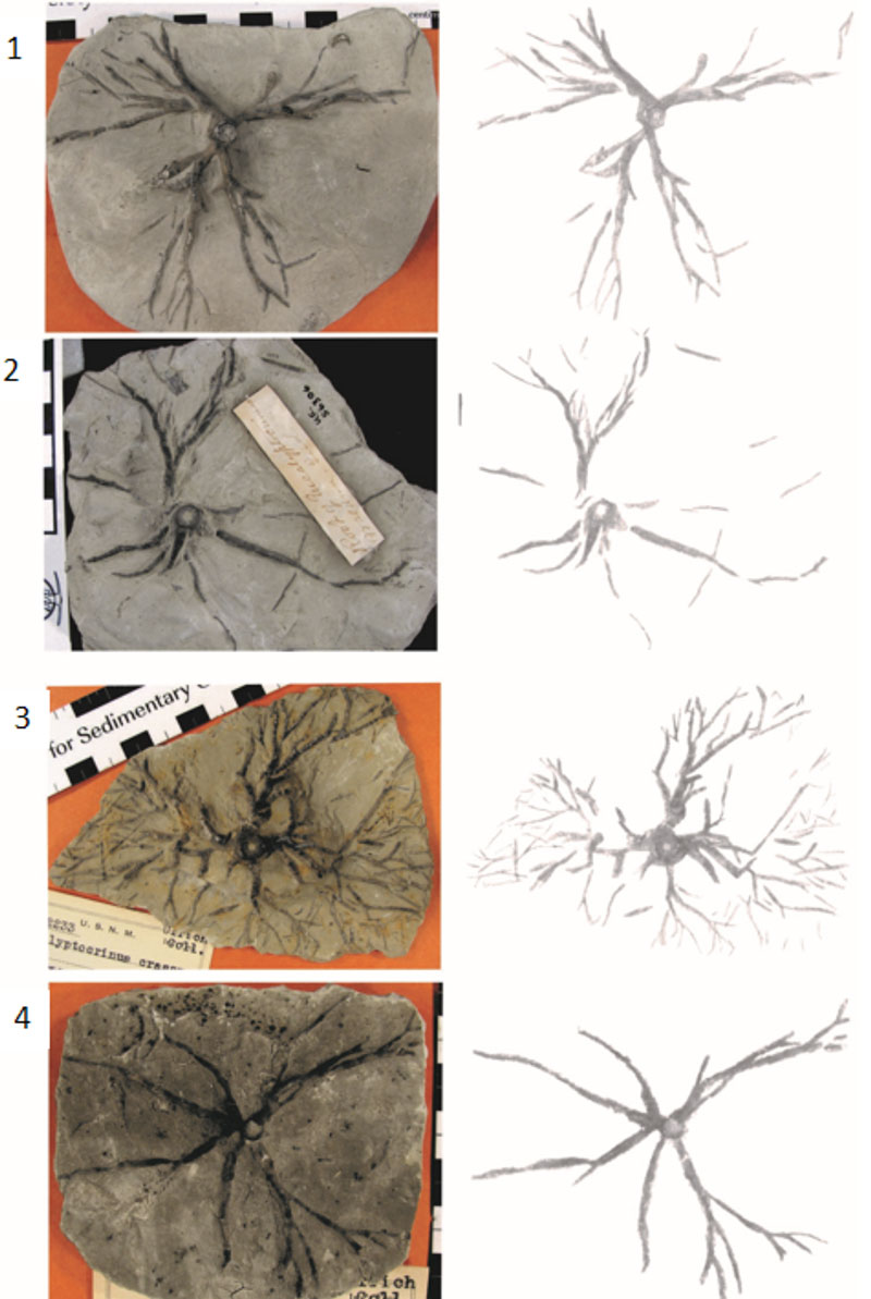
FIGURE 4. 1. Scanned image of a book (American Geosciences Institute Data Sheets, 1982). 2. Grayscale frequency distribution of image shown in 4.1. Because the background and foreground are clearly distinct, Otsu’s method works well even when applied globally with no pre-processing. The red line is the threshold chosen to segment the image. 3. Image in 4.1 treated with Otsu’s method. The details of the image shown in 4.1 are very well preserved in the treated image. 4. Checkerboard shadow illusion developed by Adelson at the Massachusetts Institute of Technology as part of the joint collaboration between the Department of Brain and Cognitive Sciences and the Computer Science and Artificial Intelligence Laboratory (CSAIL). 5. The white squares within the shadow area are incorrectly identified as dark squares by global Otsu’s method without preprocessing (Images from AGI Data Sheets and CSAIL are used with permission).
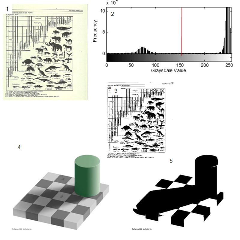
FIGURE 5. Applying local thresholding to the checker shadow illusion. The black checks and the white checks are correctly segmented.
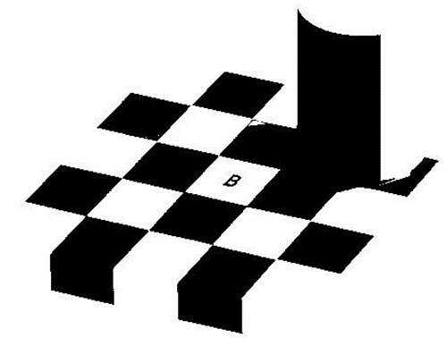
FIGURE 6. Result of the global thresholding of the image of a crinoid holdfast (see Figure 2.2). Without preprocessing there is a high level of noise (black spots).
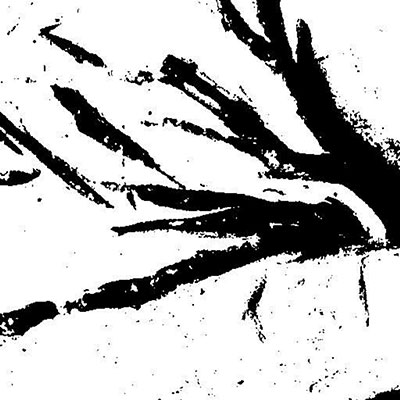
FIGURE 7. Effects of denoising. 1. The original grayscale image denoised. 2. How the denoising impacts the resulting thresholded image. Notice that there is less noise and irregular, porous edges than in Figure 6.
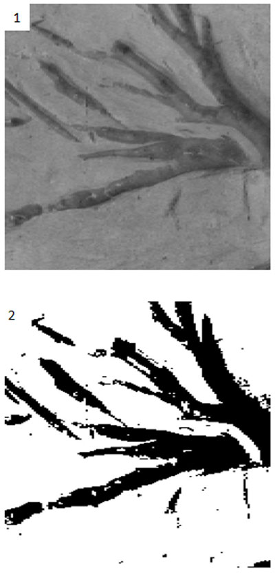
FIGURE 8. Connected component analysis. 1. The original binary image produced by preprocessing and segmentation of the tile shown in Figure 2.2. False color image of 8.1 showing the five largest objects in the image. Connected component analysis allows us to identify and remove the smaller objects. 3. Binary image after removing the smaller objects.
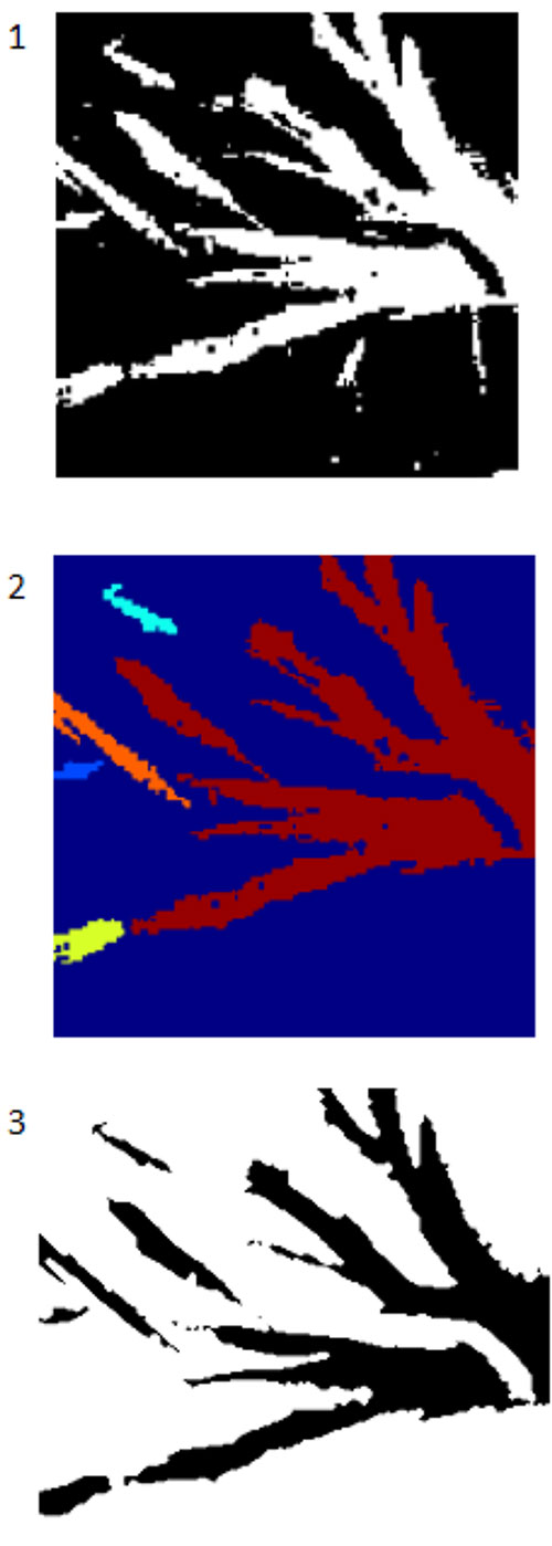
FIGURE 9. The effects of postprocessing using CC analysis and binary morphology. 1. CC analysis was applied to the denoised thresholded image in Figure 8. CC analysis has removed most of the remaining artifacts. 2. Once CC analysis is complete, binary image morphology can be used to smooth the edges of the image which better aligns with the real fossil image. 3. By applying another form of binary image morphology, an outline of the perimeter of the segmented image can be produced and the quality of the segmentation compared to the real specimen. Here we can see qualitatively that the match is very high.
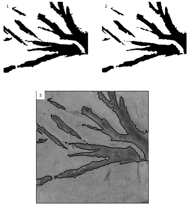
FIGURE 10. Definitions of morphometric parameters. Each branch is defined as a link between nodes (circles). Each node has an order determined by the number of nodes from the stem nodes (purple). First order nodes (red) have no nodes separating them from the stem. Second order nodes (blue) have first order nodes separating them from the stem. Third order nodes (yellow) have second order nodes separating them from the stem. The node angle is the branching angle as defined by the next order nodes. The area is the area of the branch between the nodes, which are bounded by lines perpendicular to the bisector of the node angle.
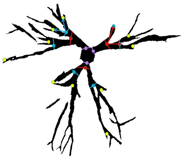
FIGURE 11. 1. Original scanned image of the bivalve Modiola from plate 8 of Murchison (1839) obtained via Google Books (TM). The digitized copy shows notable foxing. 2. Image reconstructed with thresholding of the green portion of the RGB image. This fast method of cleaning up the image for presentation and publication has removed the stains from the image.
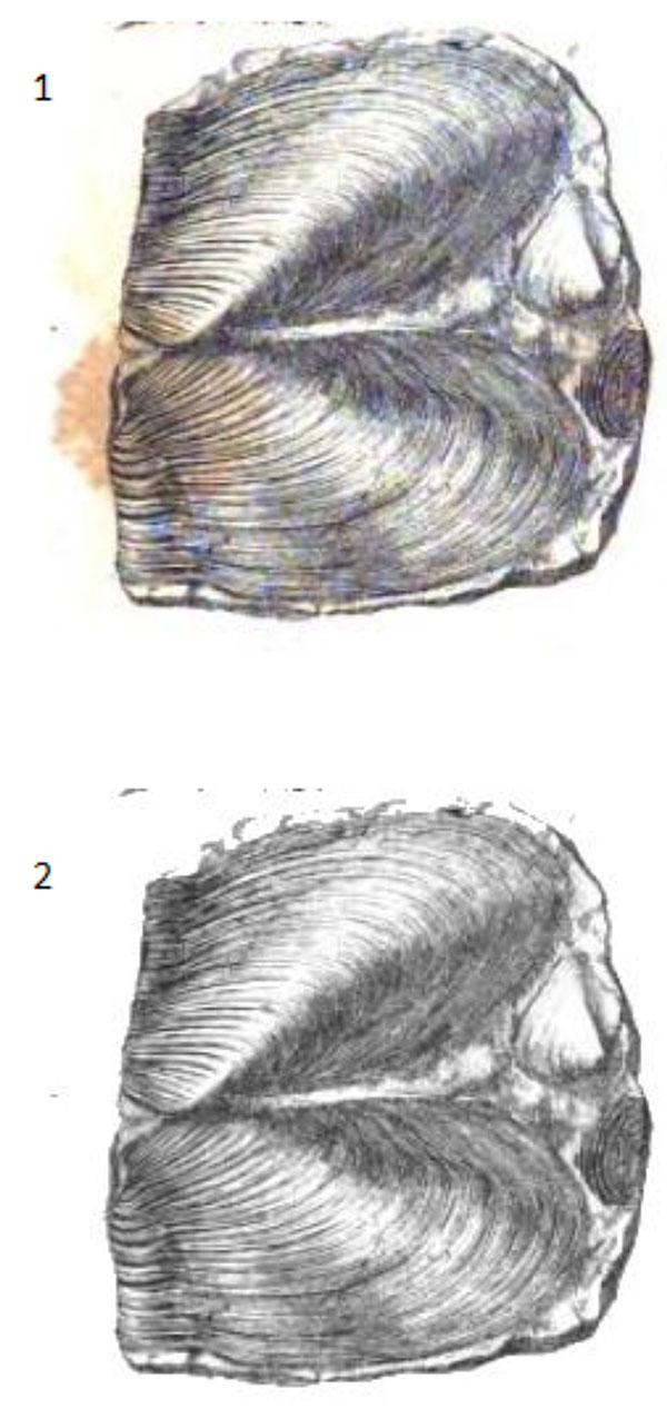
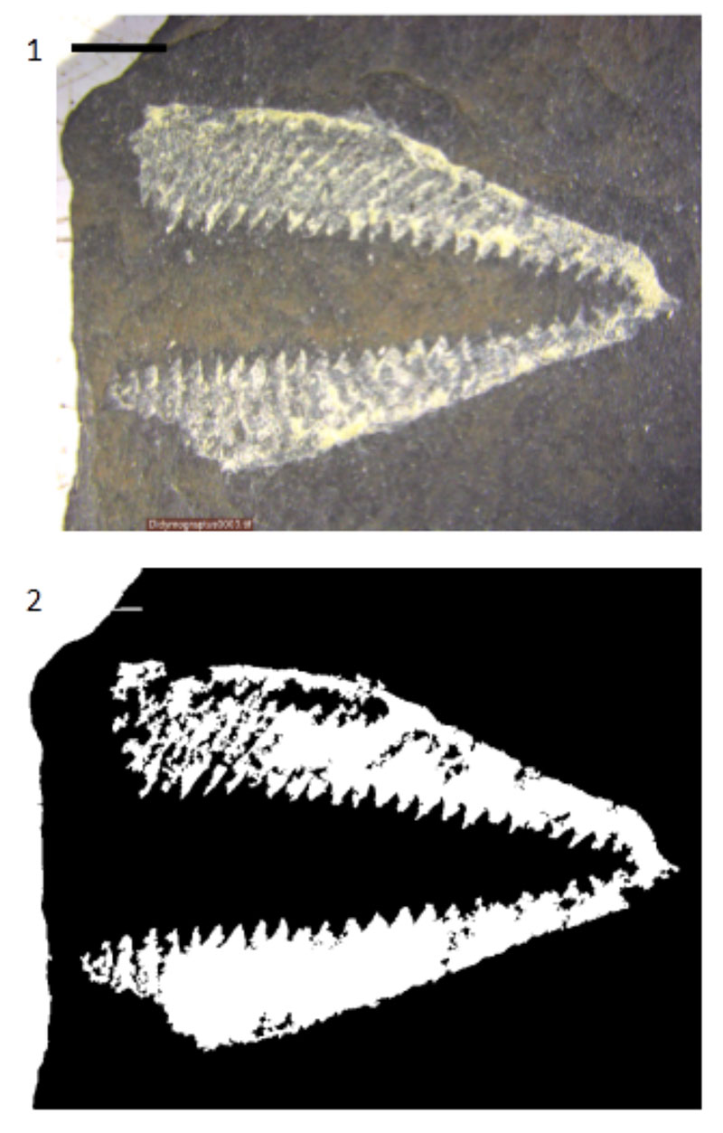
FIGURE 12. The effects of the techniques described in the paper on a graptolite rhabdosome from the University of Illinois at Chicago teaching collection, Silurian, Wales. Scale bar equals 5 mm. Processing was done on the original JPEG image. 1. Original image. 2. Segmented image.