FIGURE 1. An illustration of the taphonomic filter in the simulation, shown applied to a single taxon in a single time bin. The taxon is originally present in every locality in each region it occupies, but the taphonomic filter removes it from randomly selected localities
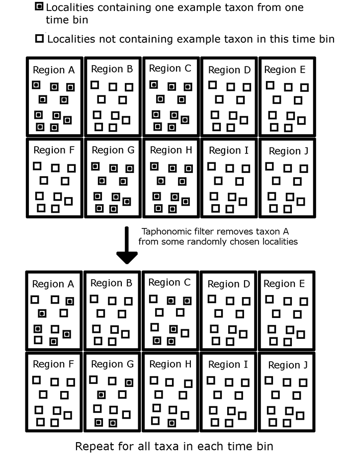
FIGURE 2. An illustration of how sampling proxies are generated in this simulation. This schematic illustrates which formations and localities in a single time bin contain fossils of at least one species of the simulated clade after application of the taphonomic filter. Formations and localities are removed at random, representing a lack of sampling. Note that the number of clade-bearing formations and localities does not necessarily equal the number of formations and localities sampled, allowing the generation of four sampling proxies.
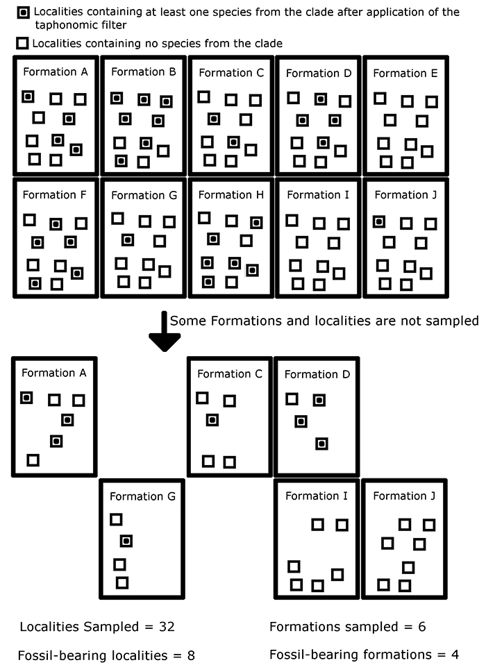
FIGURE 3. The performance of different implementations of the residual diversity estimate (RDE) under different sampling regimes. (3.1) Mean Spearman’s rho values of four implementations of the RDE using Formations as a proxy, with values of PFORM, PLOC and PTAPH variable but equal. (3.2) Mean Spearman’s rho values of four implementations of the RDE using Localities as a proxy. (3.3) Mean Spearman’s rho values of four implementations of the RDE, all using the Smith and McGowan method. (3.4) Mean Spearman’s rho values of the taxic and phylogenetic diversity estimate compared to those of the optimum implementation of the RDE. The dashed red line indicates the critical value at p=0.05. Abbreviations as in Table 1.
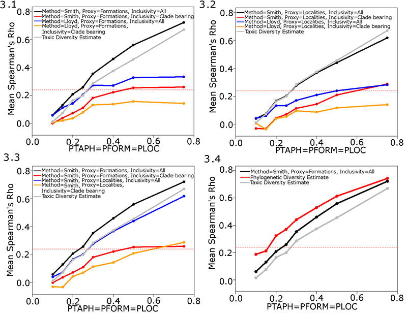
FIGURE 4. The performance of different implementations of the residual diversity estimate examining faunas with varying degrees of homogeneity. PFORM, PLOC and PTAPH are set at 0.25. The rate of dispersal is increased relative to the rate of local extinction to increase the homogeneity of the faunas. The dashed red line indicates the critical value at p=0.05. Abbreviations as in Table 1.
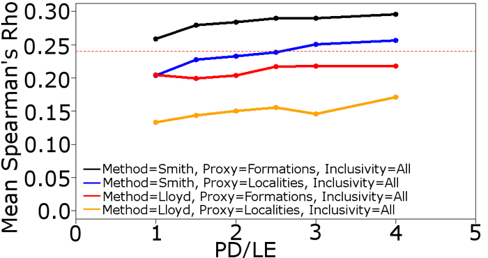
FIGURE 5. The performance of different implementations of the residual diversity estimate when a specific bias is forced to be the dominant influence. (5.1) Mean Spearman’s rho values of four implementations of the RDE using the Smith and McGowan method. PFORM and PTAPH are set at 0.9 to minimise their influence, PLOC is variable. PMIST set at 0.1. (5.2) Mean Spearman’s rho values of four implementations of the RDE using the Smith and McGowan method. LOC and PTAPH are set at 0.9 to minimise their influence, PFORM is variable. PMIST set at 0.1. The dashed red line indicates the critical value at p=0.05. Abbreviations as in Table 1.
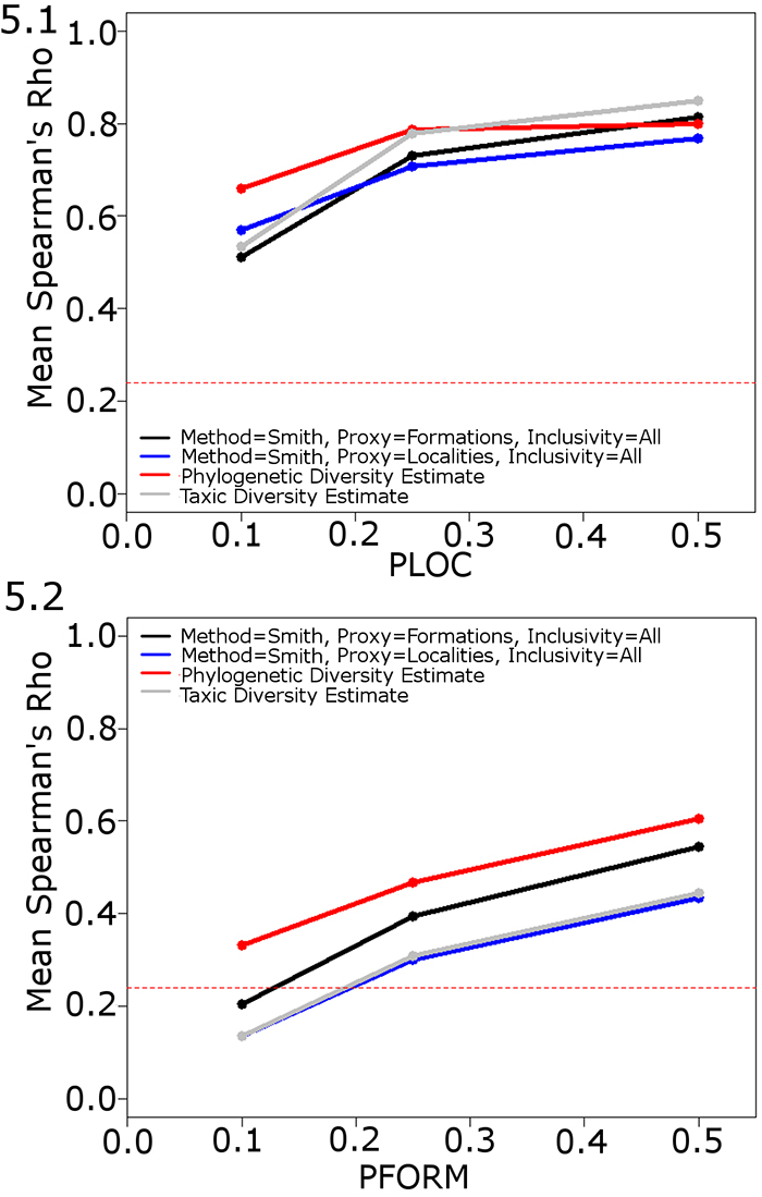
FIGURE 6. The performance of the phylogenetic diversity estimate when errors are introduced to the phylogeny. Mean Spearman’s rho values of the PDE, TDE and the best performing implementation of the RDE. PLOC, PFORM and PTAPH set at 0.25. PMIST variable. The dashed red line indicates the critical value at p=0.05. Abbreviations as in Table 1.
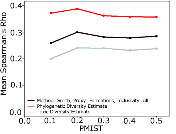
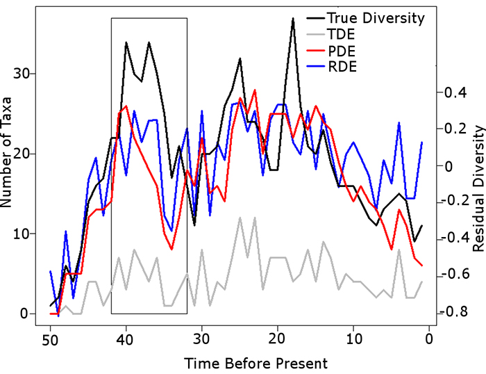
FIGURE 7. Sample simulation comparing the results of the taxic, phylogenetic and residual diversity estimates to the true diversity. PFROM, PLOC and PTAPH set at 0.25. PMIST set at 0.1. Black box highlights instance where the Signor Lipps effect has been exaggerated by the PDE; the TDE and RDE both identify the rapid diversity decrease present in the true diversity. Abbreviations as in Table 1.