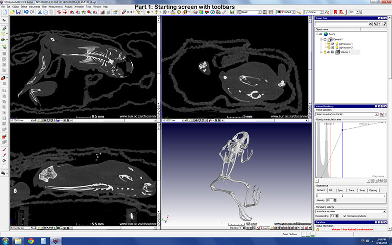
Part 1. Starting Screen with Toolbars
Part 2. Region growing
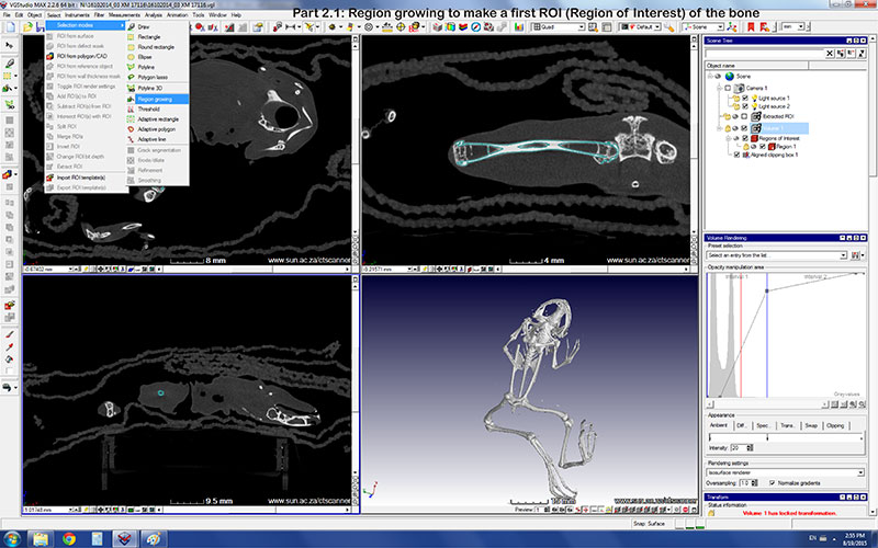
2.1. Region growing to make a first ROI (Region of Interest) of the bone.
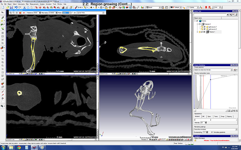
2.2. Region growing (continued).
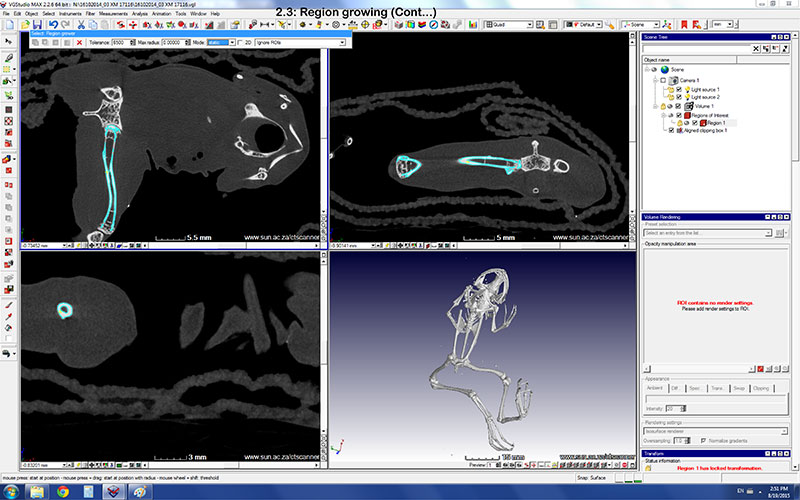
2.3. Region growing (continued).
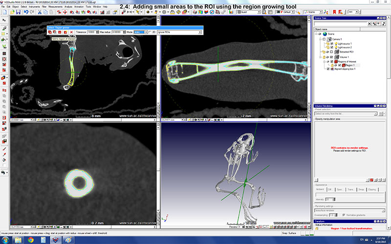
2.4. Adding small areas to the ROI using the region growing tool.
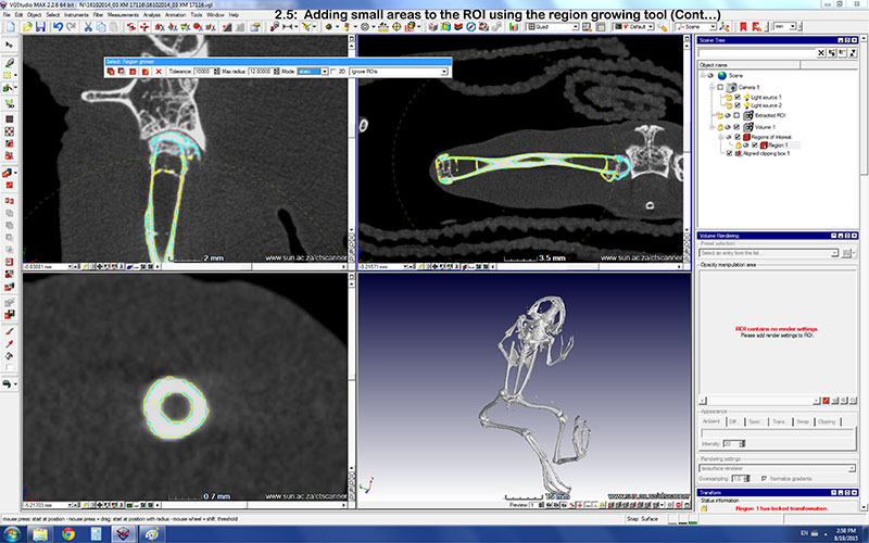
2.5. Adding small areas to the ROI using the region growing tool (continued).
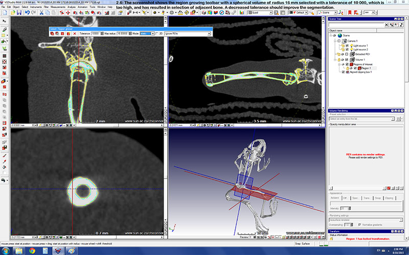
2.6. The screenshot shows the region growing toolbar with a spherical volume of radius 16mm selected with a tolerance of 10 000, which is too high, and has resulted in selection of adjacent bone. A decreased tolerance should improve the segmentation.
Part 3. Segmenting
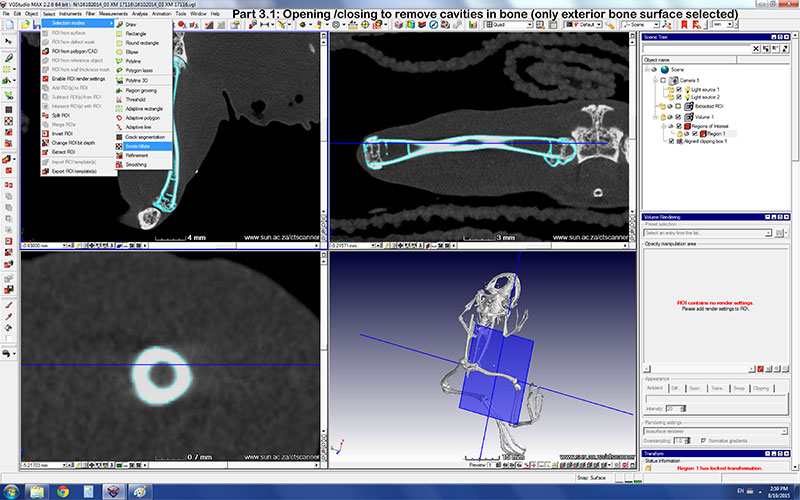
3.1. Opening/closing to remove cavities in bone (only exterior bone surface selected).
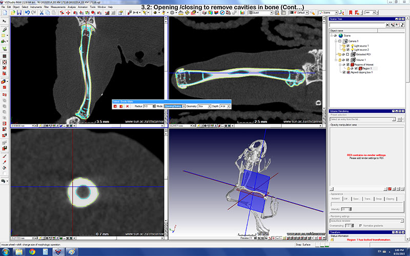
3.2. Opening/closing to remove cavities in bone (continued).
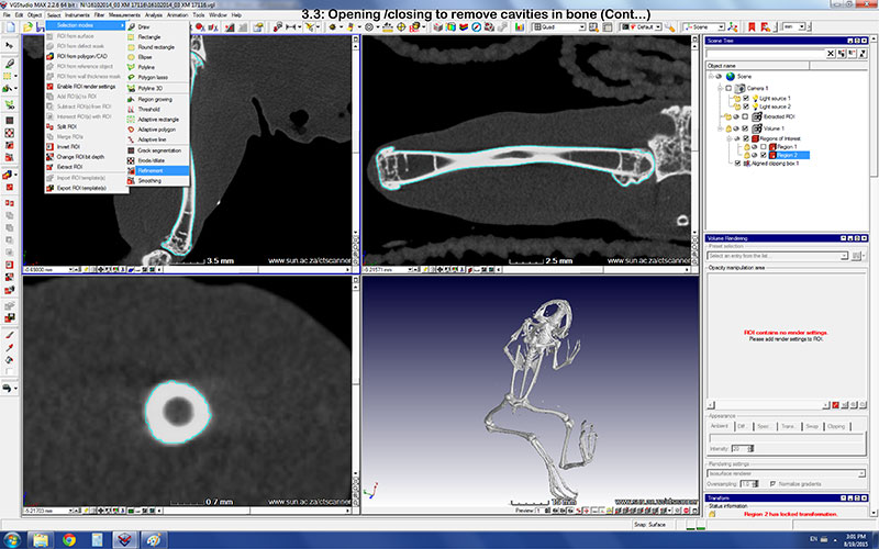
3.3. Opening/closing to remove cavities in bone (continued).
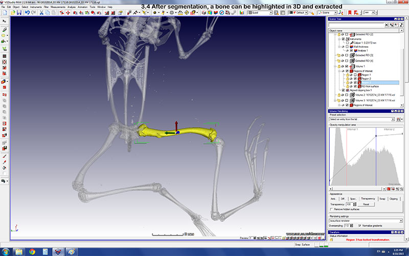
3.4. After segmentation, a bone can be highlighted in 3D and extracted.
Part 4. Setting threshold values
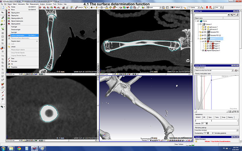
4.1. The surface determination function.
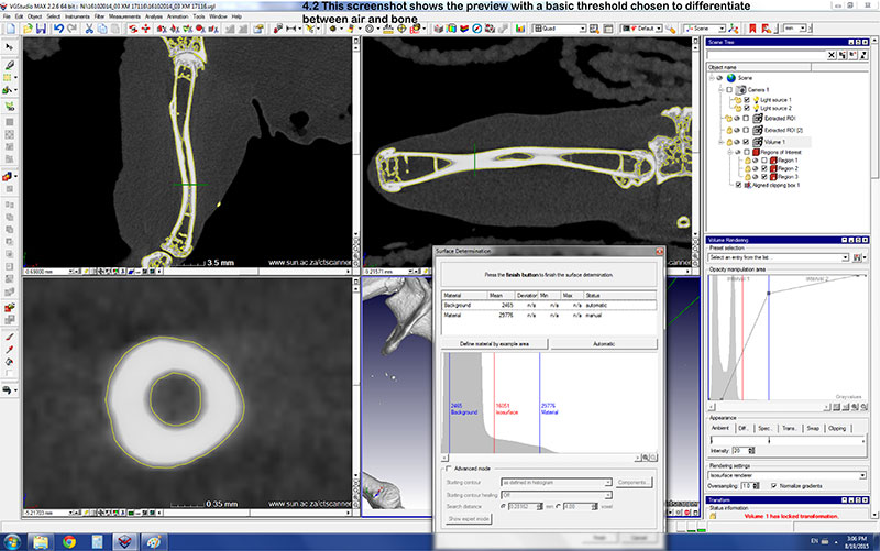
4.2. This screenshot shows the surface determination preview with a basic threshold chosen to differentiate between air and bone.
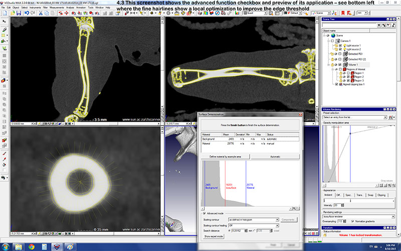
4.3. This screenshot shows the advanced function checkbox and preview of its application - see bottom left where the fine hairlines show a local optimization to improve the edge threshold.
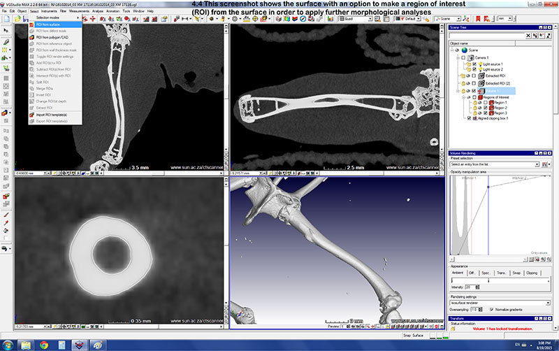
4.4. This screenshot shows the surface with an option to make a ROI from the surface in order to apply further morphological analyses.
Part 5. Wall thickness
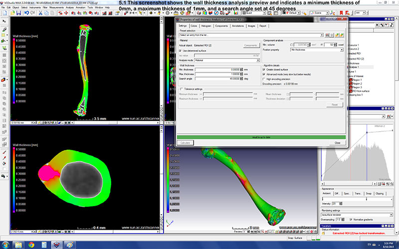
5.1. This screenshot shows the wall thickness analysis preview and indicates a minimum thickness of 0 mm, a maximum thickness of 1 mm, and a search angle set at 45 degrees.
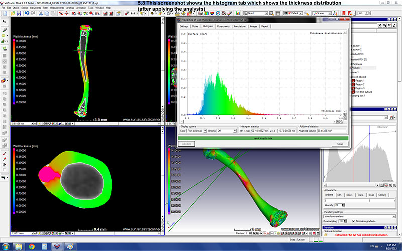
5.2. This screenshot shows the histogram tab which shows the thickness distribution (after applying the analysis).
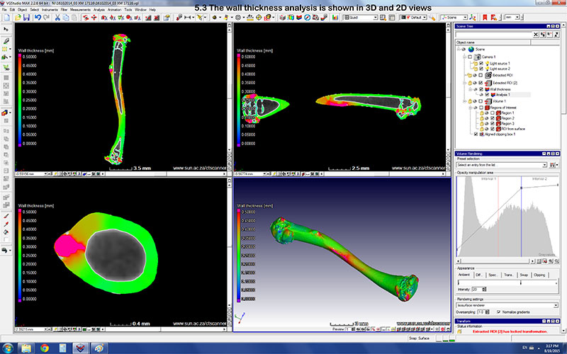
5.3. The wall thickness analysis is shown in 3D and 2D views.
Part 6. Using the virtual calipers
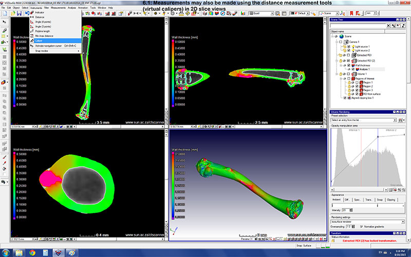
6.1. Measurements may also be made using the distance measurement tools (virtual calipers) in 2D slice views.
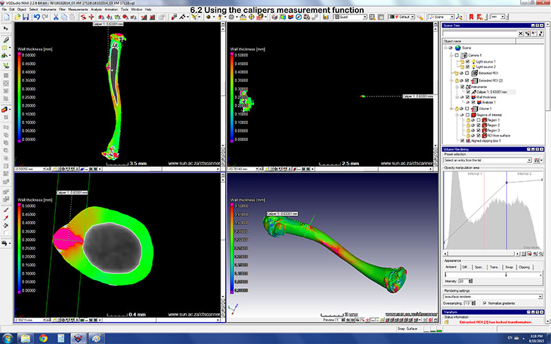
6.2. Using the calipers measurement function.
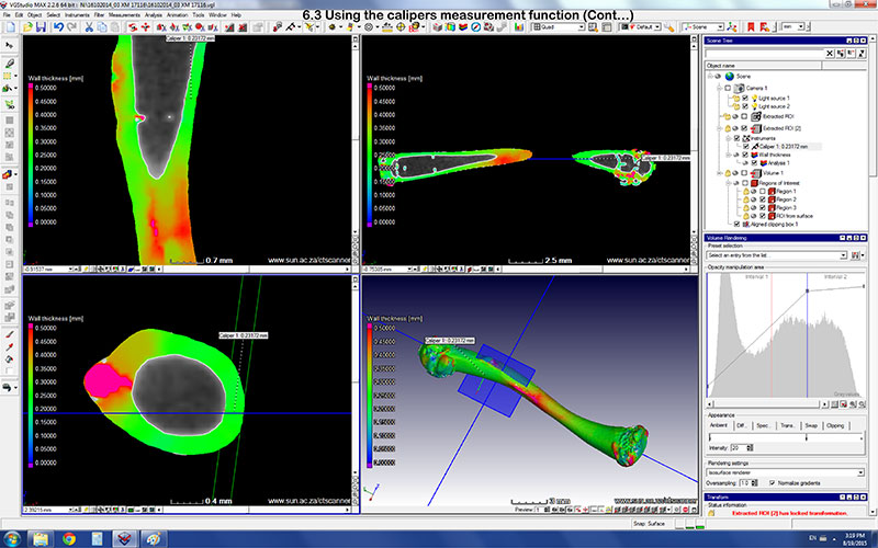
6.3. Using the calipers measurement function (continued).
Part 7. Mirror axis option
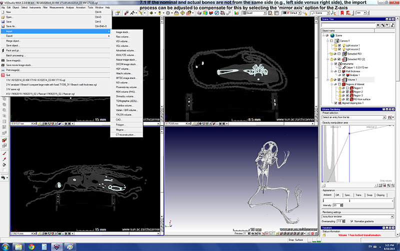
7.1. If the nominal and actual bones are not from the same side (e.g., left side versus right side), the import process can be adjusted to compensate for this by selecting the ‘mirror axis’ option for the Z-axis.
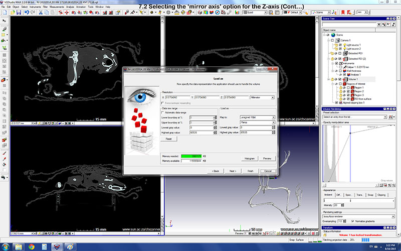
7.2. Selecting the ‘mirror axis’ option for the Z-axis (continued).
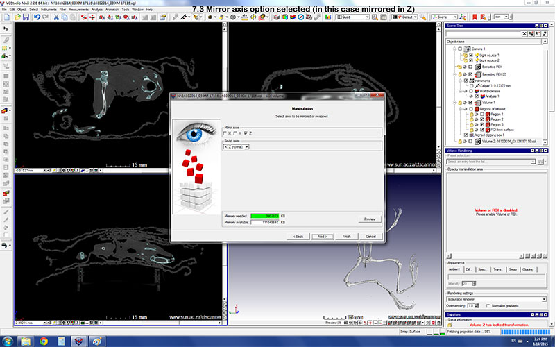
7.3. Mirror axis option selected (in this case mirrored in Z).
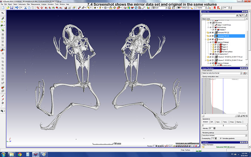
7.4. Screenshot shows the mirror data set and original in the same volume.
Part 8. Surface determination
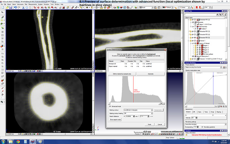
8.1. Preview of surface determimation with advanced function (local optimization shown by hairlines in slice views).
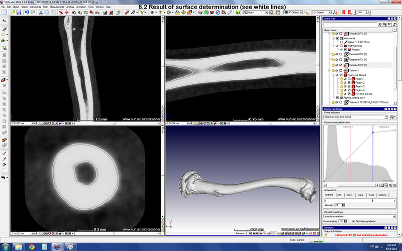
8.2. Result of surface determination (see white lines).
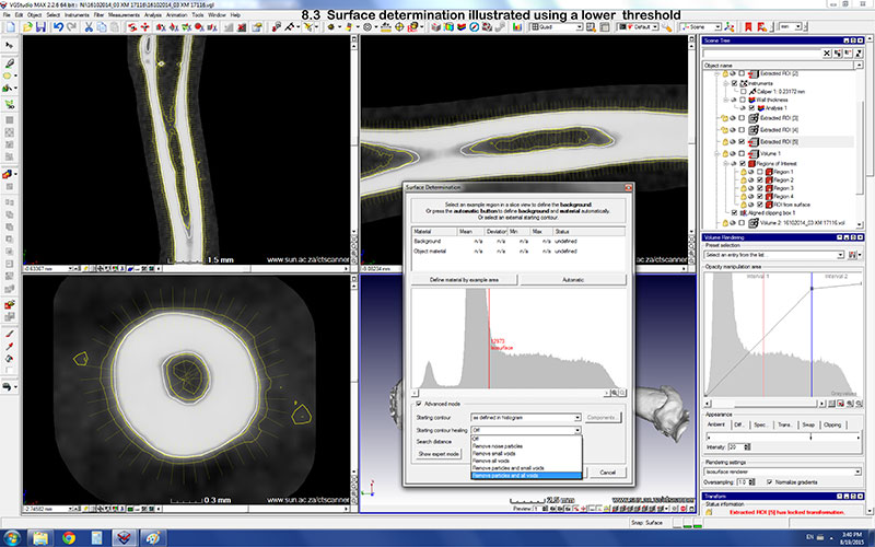
8.3. Surface determination illustrated using a lower threshold.
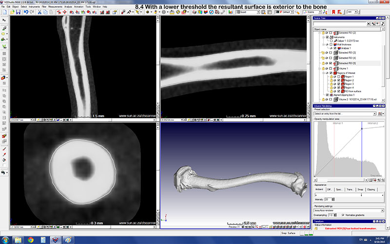
8.4. With a lower threshold the resultant surface is exterior to the bone.
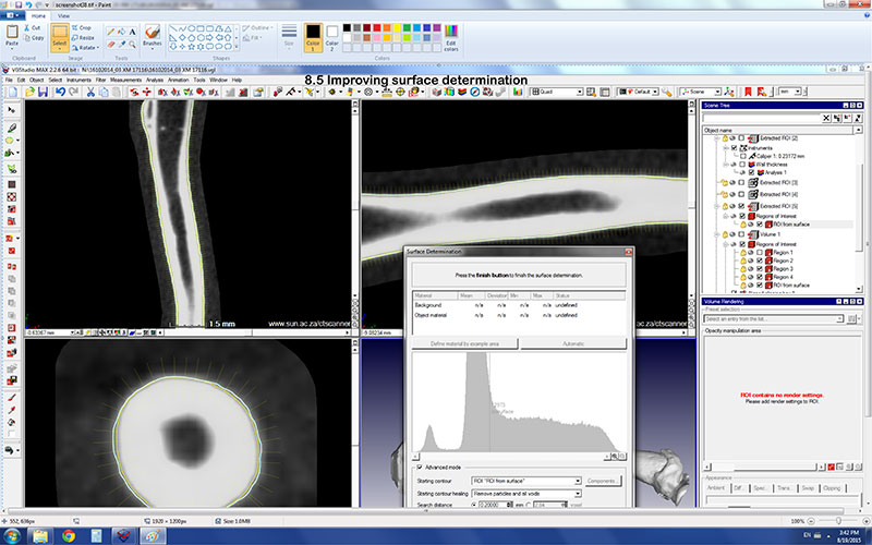
8.5. Improving surface determination.
Part 9. ‘Best-fit’ registration
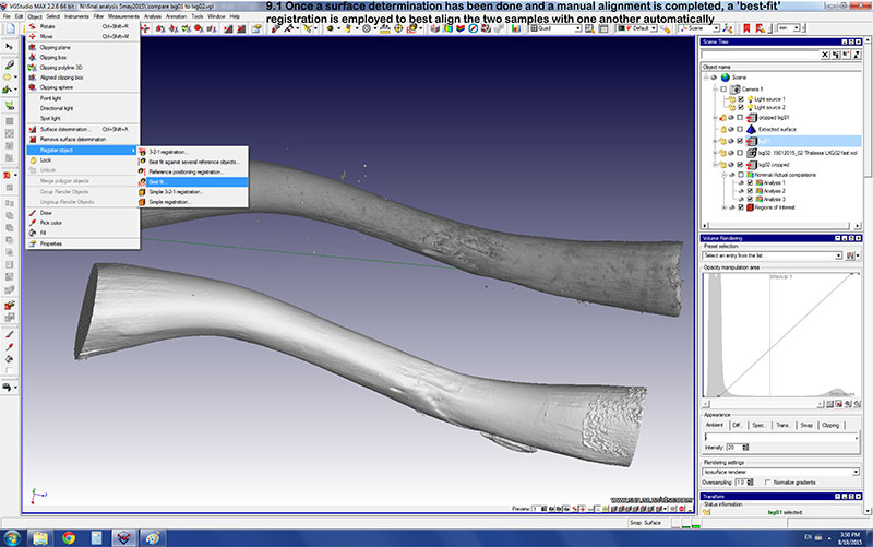
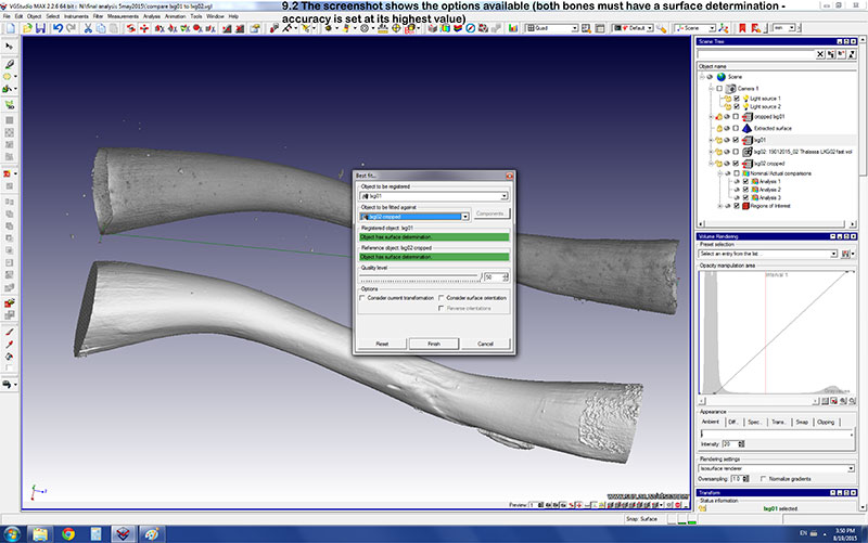
9.1. Once a surface determination has been done and a manual alignment is completed, a ’best-fit’ registration is employed to best align the two samples with one another automatically.
9.2. The screenshot shows the options available (both bones must have a surface determination -- accuracy is set at its highest value).
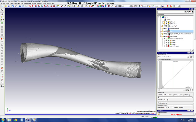
9.3. Result of a ‘best-fit’ registration.
Part 10. Nominal/Actual Comparison
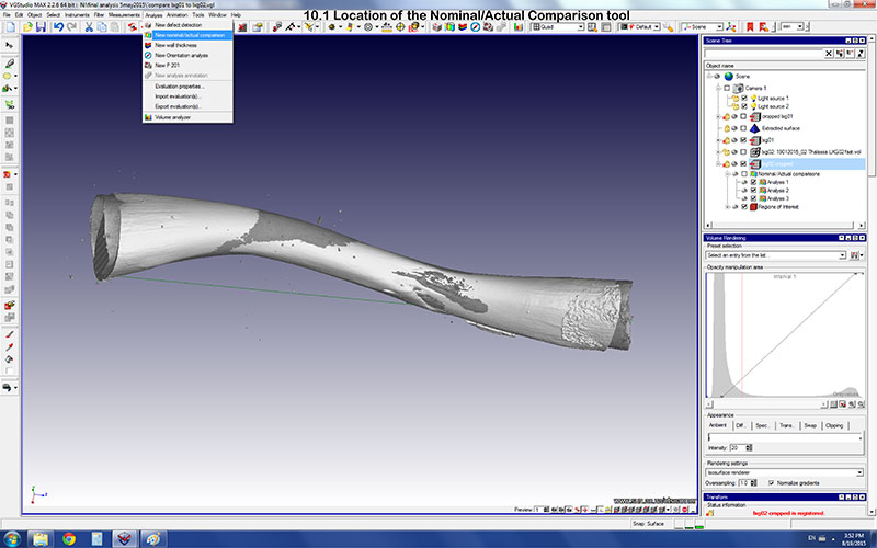
10.1. Location of the Nominal/Actual Comparison tool.
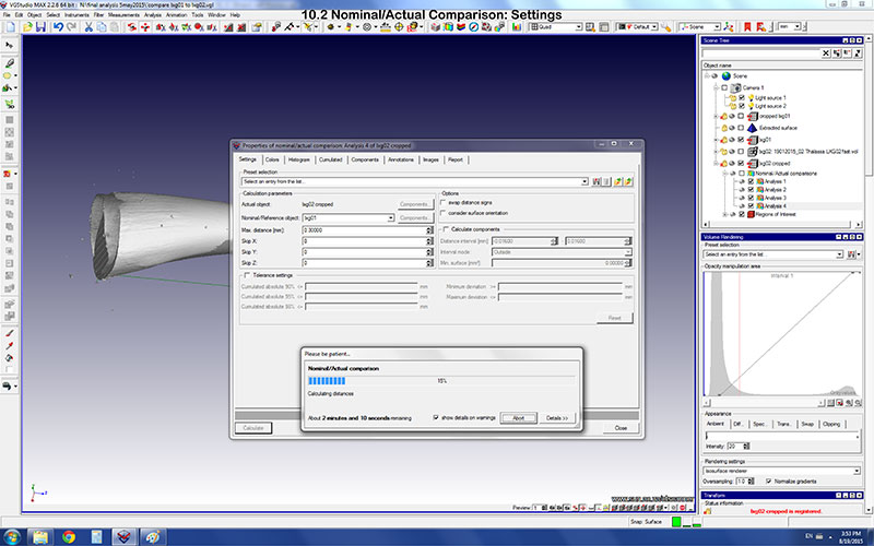
10.2. Nominal/Actual Comparison: Settings.
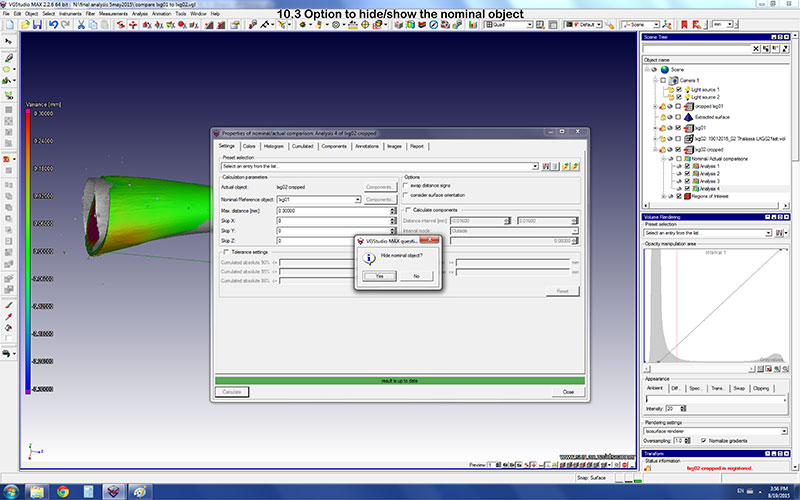
10.3. Option to hide/show the nominal object.
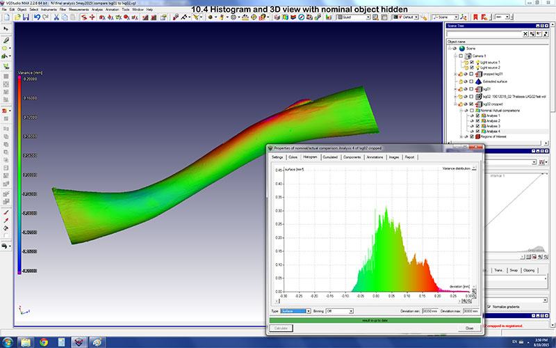
10.4. Histogram and 3D view with nominal object hidden.