FIGURE 1. Map of the northeastern coast of the USA, showing part of the northern portion of the Atlantic Coastal Plain and the location of the studied cores: BR = Bass River; C = Clayton; WL = Wilson Lake; CD = Cambridge-Dorchester; MCBR = Mattawoman Creek-Billingsley Road. The New Jersey Coastal Plain is the northern section of the Salisbury Embayment. In outcrop, the Fall Line marks the change from Precambrian and Paleozoic rocks of the Piedmont province in the west to the relatively undeformed, slightly dipping Mesozoic and Cenozoic sediments of the Coastal Plain in the east (Gibson and Bybell, 1994). For visual ease, the New Jersey Coastal Plain and the Salisbury Embayment labels are delineated offshore.
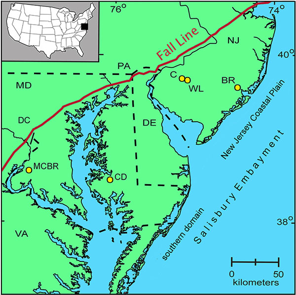
FIGURE 2. Specimen storage in the Naturalis (Leiden, NL) fossil holoplanktic mollusk collection.
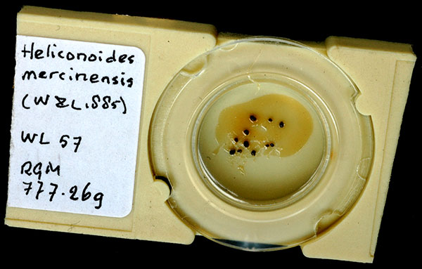
FIGURE 3. Altaspiratella elongatoidea (Aldrich, 1887). 1, Wilson Lake section, sample 31, depth 100.89-100.95 m, RGM 777 230; apertural view. 2, Clayton section, sample 9, depth 91.44-91.4 m; RGM 777 308a; apertural view. 3-4, Wilson Lake section, sample 42, depth 104.24-104.30 m; RGM 777 251a, 3: apertural view, 4: apical view.

FIGURE 4. Altaspiratella elongatoidea (Aldrich, 1887). Computed tomography (CT) scan of the specimen pictured in Figure 3.3-4, resolution 1.6 micrometer/voxel, 165 kV, detector exposure timing 750 ms. For the interactive version, download the PDF to your hard drive or desktop and open in Acrobat or enable the 3D option in Acrobat in your Internet browser. By clicking on the image, the interactive 3D model is activated, and the reader can use the mouse to rotate the specimen and change magnification.
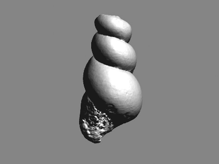
FIGURE 5. Heliconoides mercinensis (Watelet and Lefèvre, 1885). 1-3, Wilson Lake section, sample 27, depth 99.67-99.73 m, RGM 777 223a; 1: apical view, 2: apertural view, 3: umbilical view.
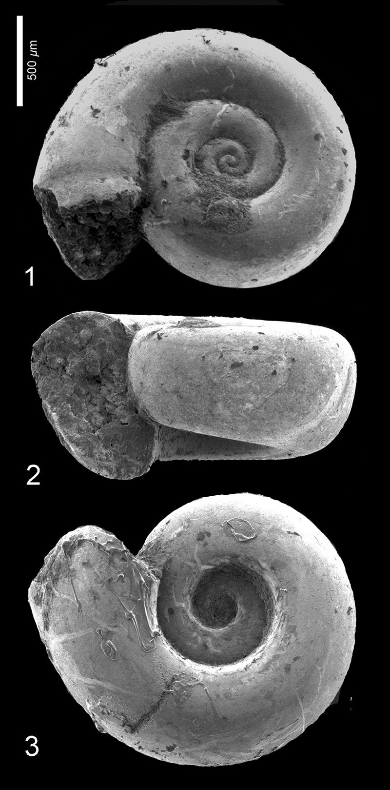
FIGURE 6. Heliconoides mercinensis (Watelet and Lefèvre, 1885). Computed tomography (CT) scan of the specimen pictured in Figure 5.1-3. Resolution 1.9 micrometer/voxel, 165 kV, detector exposure timing 750 ms. For the interactive version, download the PDF to your hard drive or desktop and open in Acrobat or enable the 3D option in Acrobat in your Internet browser. By clicking on the image, the interactive 3D model is activated, and the reader can use the mouse to rotate the specimen and change magnification.
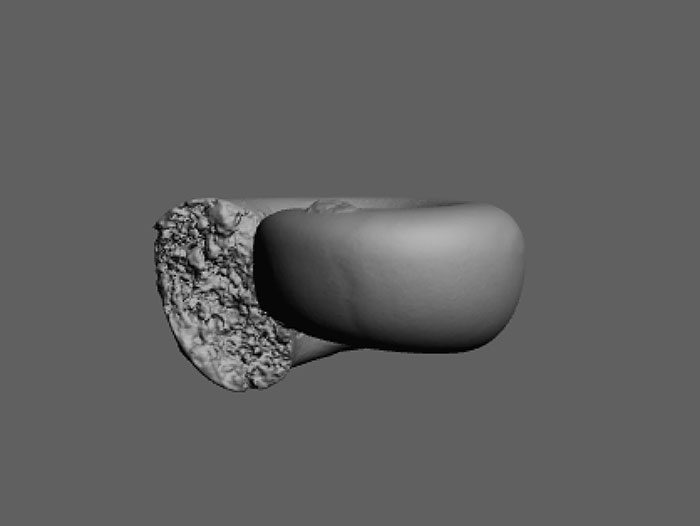
FIGURE 7. Limacina aegis Hodgkinson in Hodgkinson, Garvie and Bé, 1992. 1, Clayton section, sample 19, depth 94.55-94.58 m, RGM 777319a; apertural view. 2, Clayton section, sample 21, depth 95.07-95.10 m, RGM 777 323; apertural view. 3-4, Wilson Lake section, sample 34, depth 101.80-101.86 m, RGM 777 236a; 3: apical view, 4: apertural view. 5-6, Wilson Lake section, sample 52, depth 07.08-107.11 m, RGM 777 264a; 5: apertural view, 6: umbilical view. 7-9, Wilson Lake section, sample 63, depth 108.20-108.26 m, RGM 777 283 (specimen lost); 7: apical view, 8: apertural view; 9: umbilical view. 10-11, Cambridge-Dorchester section, sample 15, depth 220.22-220.28 m, RGM 777 338; 10: apical view, 11: apertural view.
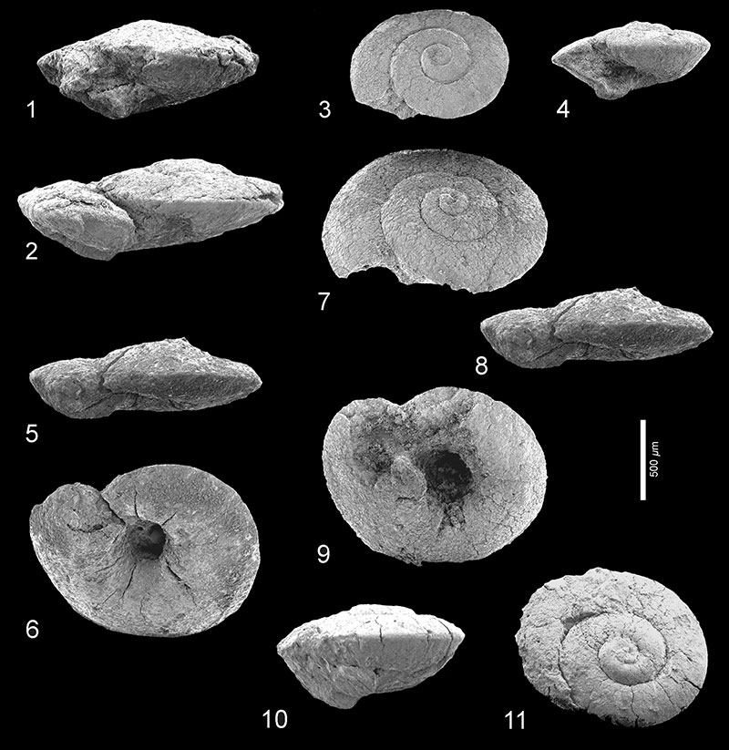
FIGURE 8. Limacina aegis Hodgkinson in Hodgkinson, Garvie and Bé, 1992. Computed tomography (CT) scan of specimen RGM 777.264b, which has the same locality data as the specimen in Figure 7.5-6. Resolution 2.0 micrometer/voxel, 165 kV, detector exposure timing 750 ms. For the interactive version, download the PDF to your hard drive or desktop and open in Acrobat or enable the 3D option in Acrobat in your Internet browser. By clicking on the image, the interactive 3D model is activated, and the reader can use the mouse to rotate the specimen and change magnification.
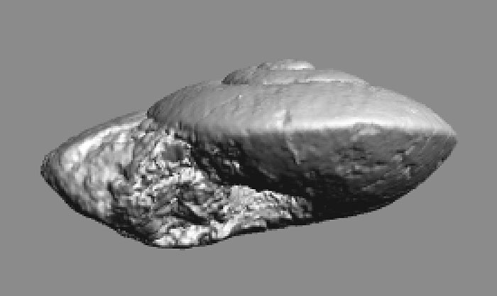
FIGURE 9. Limacina novacaesarea Janssen and Sessa sp. nov. 1-3, Holotype, Wilson Lake section, sample 24, depth 98.76-98.82 m, RGM 777 219; 1: apical; view, 2: apertural view, 3: umbilical view. 4-6, Paratype 1, Wilson Lake section, sample 22. Depth 98.15-98.21 m, RGM 777 215a; 4: apical view, 5: apertural strongParatype 2, Wilson Lake section, sample 27, depth 99.67-99.73 m, RGM 777 225; apertural view of poorly preserved, slightly depressed specimen.
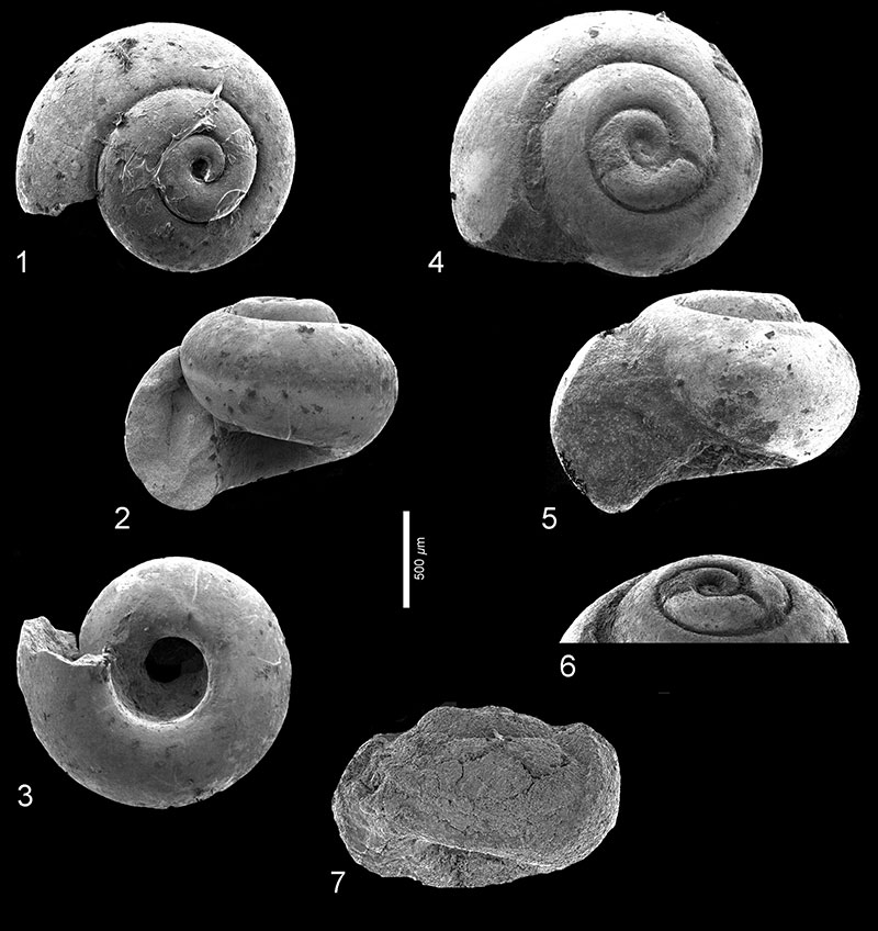
FIGURE 10. Limacina novacaesarea Janssen and Sessa sp. nov. Computed tomography (CT) scan of the specimen pictured in Figure 9.1-3. Resolution 4.0 micrometer/voxel, 185 kV, detector exposure timing 750 ms. For the interactive version, download the PDF to your hard drive or desktop and open in Acrobat or enable the 3D option in Acrobat in your Internet browser. By clicking on the image, the interactive 3D model is activated, and the reader can use the mouse to rotate the specimen and change magnification.
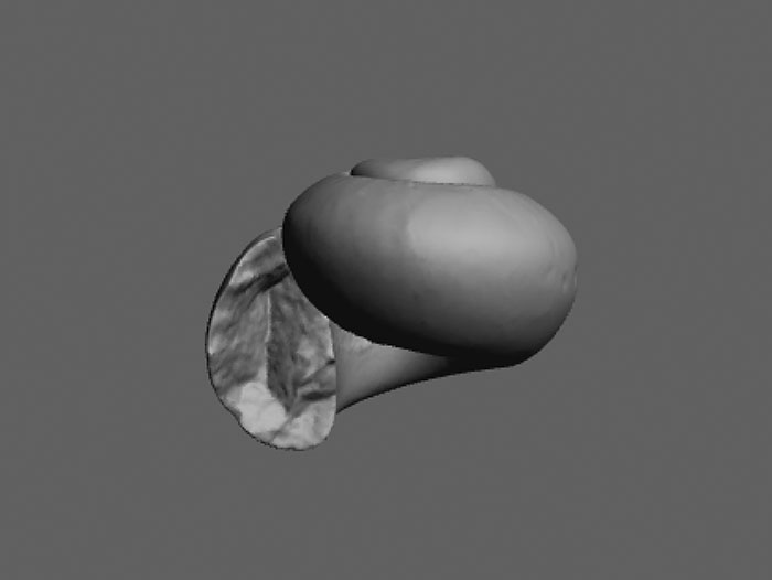
FIGURE 11. Limacina sp. 1. 1-3, Wilson Lake section, sample 37, depth 102.72-102.78 m, RGM 777 241; 1: apical view, 2: apertural view, 3: umbilical view. 4-5, Wilson Lake section, sample 50, depth 106.68-106.74 m, RGM 777259a; 4: apical view, 5: apertural view. 6, Wilson Lake section, sample 40, depth 103.02-103.08 m, RGM 777248; apical view.
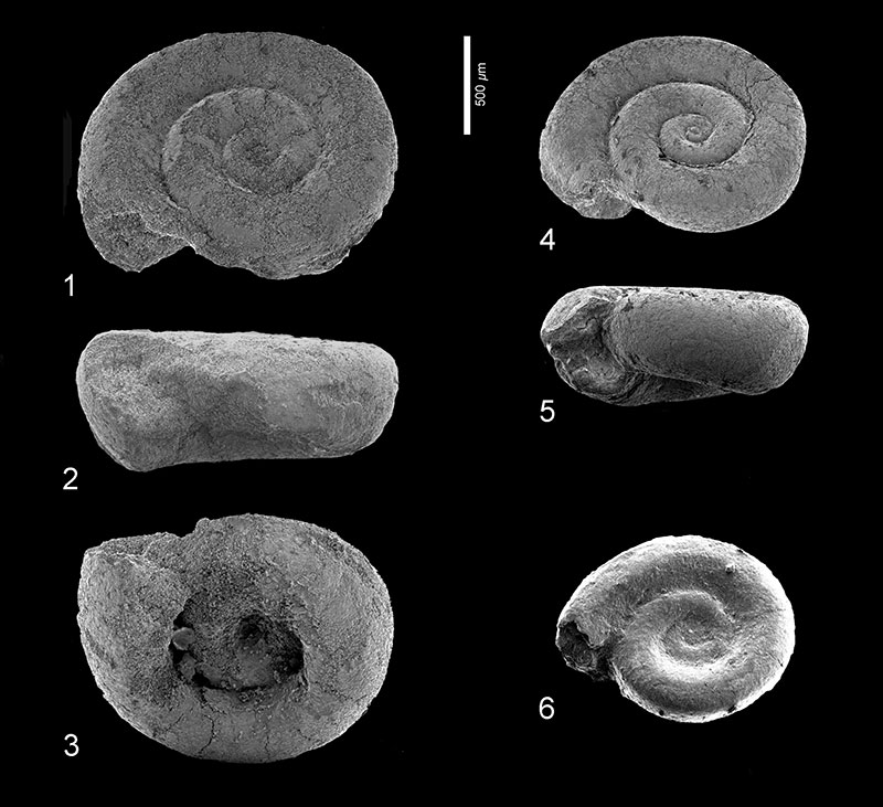
FIGURE 12. Limacina sp. 1. Computed tomography (CT) scan of the specimen pictured in Figure 11.1-3. Resolution 4.9 micrometer/voxel, 145 kV, detector exposure timing 750 ms. For the interactive version, download the PDF to your hard drive or desktop and open in Acrobat or enable the 3D option in Acrobat in your Internet browser. By clicking on the image, the interactive 3D model is activated, and the reader can use the mouse to rotate the specimen and change magnification.
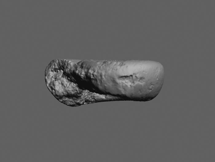
FIGURE 13. Limacina sp. 2. 1-2, Cambridge-Dorchester section, sample 26, depth 222.61-222.62 m, RGM 777 345; 1 : apical view, 2: apertural view.
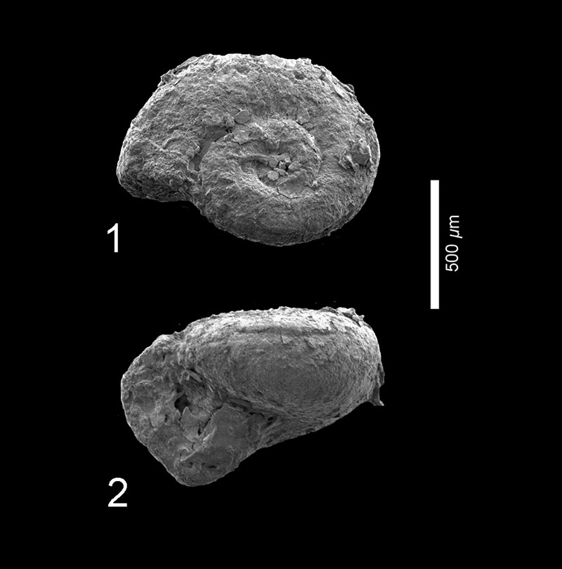
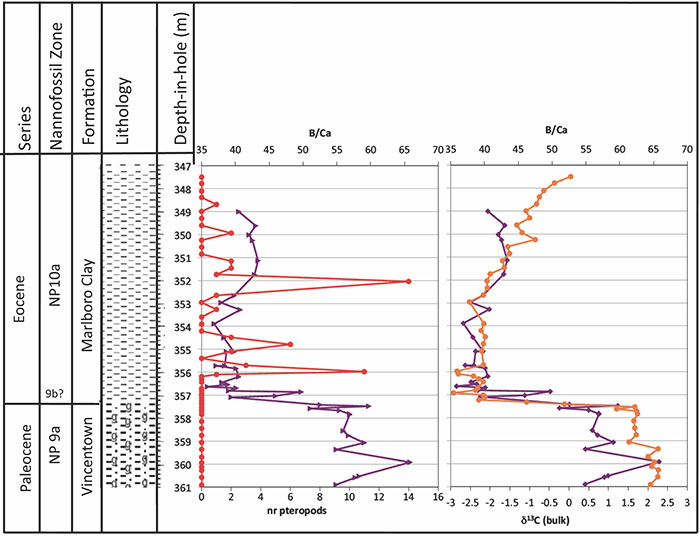
FIGURE 14. Stratigraphy and lithology for the Bass River core, after Stassen et al., 2015. The number of pteropods recognized (red) is compared to the B/Ca values (purple) in the planktonic foraminiferal genus Acarinina, a surface-water (mixed layer) dweller (Babila et al., 2016), and with δ13C values of bulk carbonate (orange), indicating the location of the carbon isotope excursion (Stassen et al., 2015). The change in B/Ca is interpreted as reflecting a decline in pH by ~0.3-0.4 pH units (Babila et al., 2016). The irregularity of pteropod distribution is likely because they were transported to these sites, and do not represent an in situ population.