FIGURE 1. Simplified structure of the RNames Database (rnames.luomus.fi/). The database contains eight related tables (blue and red objects) of which the object “Relations” is central. In “Relations” correlated stratigraphic units are listed by reference. Three output tables (yellow objects) list time binned stratigraphic units based on a search algorithm that uses “Relations” via R-Package RMySQL (the scripts are available under github.com/bjoekroe/RNames). Global Stages after Cooper et al. (2012). Abbreviations: ID, identifier; StS, Stage Slice (Bergström et al., 2009); TS, Time Slice (Webby et al., 2004)
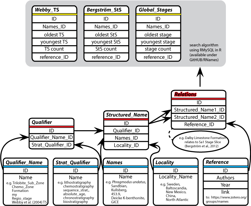
FIGURE 2. Structure of algorithm for time binning of stratigraphical units of the RNames Database (available under github.com/bjoekroe/RNames). Time bins are selected via three correlation routes (colour codes) and six rules resulting in six tables with referenced bins from which only those are selected which are most precise (i.e., range through lowest number of bins). Abbreviations: bio.unit, biostratigraphic unit; non-bio. unit, non-biostratigraphic unit. Colour code: red, correlation exclusively based on biostratigraphy; orange; correlation indirectly based on biostratigraphy; yellow, correlation based on direct or indirect assignments to time bins. -> arrow refers to referenced relations in RNames.
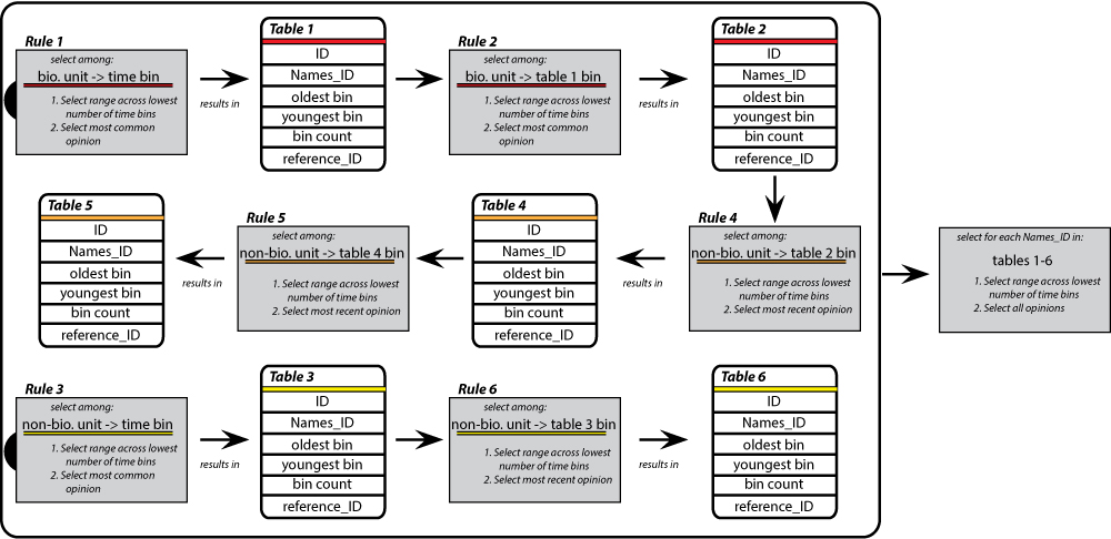
FIGURE 3. Example of the time binning of the Plectodina tenuis conodont-zone into Stage Slices (StS, Bergström et al., 2009) based on records of referenced relations in RNames and on the binning algorithm (see text and Figure 2). The P. tenuis zone is binned into the StS Sa2 time bin because three references relate the P. tenuis Zone exclusively to the Baltoniodus alobatus conodont zone, which is related to StS Sa2, based on reference 9 (Ainsaar et al., 2010). (see text for further explanation). Red circles denote selected references. Red lines denote selected relations. 1Webby et al. (2004); 2Cooper et al. (2012); 3Sweet (1984); 4Saltzman et al.(sup); 5Lehnert et al. (2005); 6Goldman et al. (2007); 7Sell et al. (2015); 8 Korén et al. (2006), 9Ainsaar et al. (2010); 10Bergström et al. (2009); 11Sennikov et al. (2014); 12Kanygin (2010); 13 (Bergström et al., 2012).
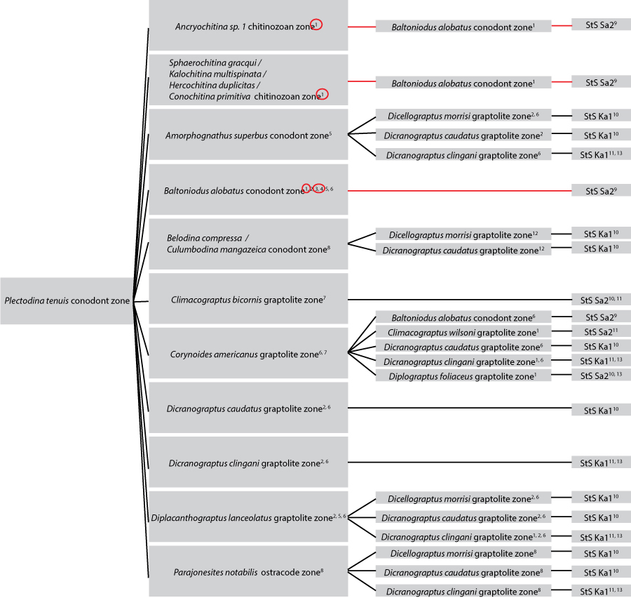
FIGURE 4. Ordovician genus-level diversity trends of PaleobioDB occurrence data, based on three different time binning approaches. 1. Total mean standing diversity (after Cooper, 2004). 2. Rarefied diversity with time bins of < 100 collections culled, with quota 600. Diamonds, two-time-bin resolution; triangles, one-time bin resolution; stars, all collections. Red, Global Stages after Cooper et al. (2012), green; Stage Slices, Bergström et al. (2009); blue, Time Slices, Webby et al. (2004). Error bars reflect 95% confidence interval.
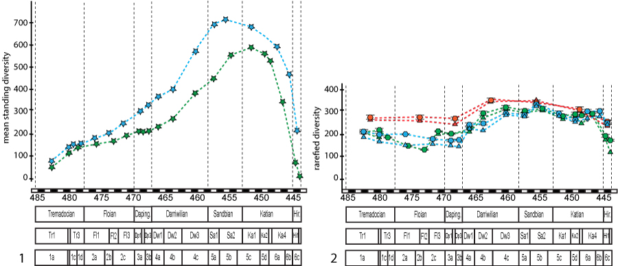
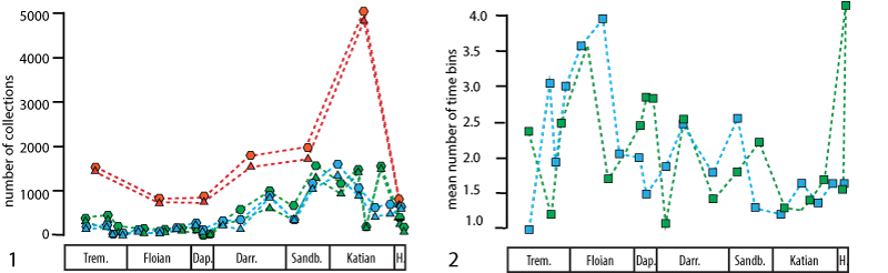
FIGURE 5. Quality of PaleobioDB data used for diversity calculations. 1. Number of collections available per time bin. 2. Mean stratigraphic range of collections through time bins. Diamonds, two-time-bin resolution; triangles, one-time bin resolution; squares, all collections. Red, Global Stages after Cooper et al. (2012), green; Stage Slices, Bergström et al. (2009); blue, Time Slices, Webby et al. (2004).