

APPENDIX 1.
Instructions for installing R, the package logspiral, and choosing a spiral for the ventral valve of the brachiopod LR-F1.
R (version >= 4.0.1) must be first installed (downloads at https://w.w.w.r-project.org/).
Download and extract the supplemental file logspiral.zip as a folder, or the supplemental tarball file: logspiral_0.9.5.tar.gz
On Windows operating system, install the folder or the tarball using the R package devtools:
library(devtools)
install_local(path="your path name\\logspiral",type="source",
force=TRUE, repos=NULL)
or
library(devtools)
install_local(path="your path name\\logspiral_0.9.5.tar.gz",
type="source", force=TRUE, repos=NULL)
If not already installed, devtools can be installed from the R command line by typing
install.packages("devtools")
Type library(logspiral)in your R session window to run the package.
Choosing a Spiral for the LR-FR1 Ventral Valve.
First, advice on outlines and the number of coordinates points. When a biological outline is digitized with less than 100 points then an L1 fit is usually the only option for a spiral. There is not enough data to fit and compare more complex spirals. A cautionary 150 to 200 outline points should be digitized before checking spirals and extracting spiral deviations. Depending on study objectives, and more knowledge on spirals fitted, the number of points can be reduced (or increased). Growth regressions or prominent zig-zags in an outline need special care as spiral fitting works well with accretion mostly in one direction.
The data for LR-FR1 is in the logspiral Supplemental Material package. The following commands were used to access the
data and to choose the L2 spiral for this valve (300 equally spaced coordinate points).
library(logspiral)
doSetupGraphics() # creates four graphic windows, but only in Windows
# alternatively, type dev.new() four times
#
data (exLaqueus)
x.df <- exLaqueus # makes a copy of the data
#
# extract the specimen F1 and its ventral valve coordinates
#
x1.df <- x.df[x.df$specimen=="F1", ]
x <- x1.df$x[x1.df$valve=="ventral"]
y <- x1.df$y[x1.df$valve=="ventral"]
#
# flip the valve so accretion tracks anticlockwise, and
# is in the positive quadrant (avoids negative spiral parameters)
x <- -1*x + 100
#
## fit an L1 spiral and plot the spiral deviations
# because a starting location is not provided for the spiral axis
# you will be asked to supply one by clicking on a graphics window
# Choose inside the valve, nearer to the umbo or posterior of the valve
#
xs1 <- fitAnyLinear(x=x,y=y, plot.deviations=T)
#
# compute Wavelet and Fourier deviation features
#
z <- computeL1DeviationFeatures(x= x, y=y, plot.it=T)
#
# compare these features to the catalogue, but no printing
# or saving of results (see help for more detail on function)
#
compareFeaturesToCatalogue(spiral.features=z,
plot.detail=TRUE, output.results=F)
#
## fit an L2 spiral, but first find the location of spiral change
xcheckL2 <- fitCheckL2Spiral(x=x, y=y, plot.detail=F)
#
# should highlight at or near the 251st coordinate as
# the spiral change on the outline
#
xL2 <- fitAnyLinear(x=x,y=y, m=251,
axis.start=c(55,12), plot.deviations=T)
#
# print to the console the estimate of the standard deviation of
# spiral deviations.
#
xL2$parameters2[1]
#
## the L3 spiral fit, first find the location of the second spiral change
#
xcheckL3 <- fitCheckL3Spiral(x=x, y=y,m=251, plot.detail=F)
#
# should highlight at or near the 70th coordinate as second change point
# and an estimate of the spiral axis location.
#
xL3 <- fitAnyLinear(x=x,y=y, m=c(70,251),
axis.start=c(60,12), plot.deviations=T)
#
## the linear to bent cable spiral fit
#
xL2QL <- fitLinear2BentCable(x=x, y=y, m=c(70,251), axis.start=c(57,12),
start.values=c(a0=3.7, k0=48, k1=45, k2=55, g=0.3, kappa=2),
plot.deviations = T, plot.fit = T)
#
# type help(logspiral) or ?logspiral to view all functions
# and further explanations of the package.
#
# Cubic (C) spiral fit, subsequently rejected as an unstable fit
# (note that this use requires an initial axis as screen input)
#
xCubic <- fitCubic(x=x,y=y, quadratic.start=0.005,
cubic.start=-0.01, plot.deviations=T, plot.fit=T)
#
# Quartic (QQ) spiral fit also rejected, but this time because of more
# variability in the spiral deviations (compared to the L2, L3 fits)
#
xQuartic <- fitQuartic(x=x,y=y, quadratic=0.005, cubic=0.01,
quartic=-0.005,plot.deviations=T)
#
# L2 is the final choice of spiral for this outline
#
## Fourier spectrum of the L2 spiral deviations
#
doSpectrum(xL2$deviations, wave1=0, wave2=20)
#
# Wavelet scalogram of the L2 spiral deviations.
#
xL2wavelets <- computeDeviationWavelets(xL2)
#
# see text for explanation and help(computeDeviationWavelets)in logspiral
# ----------------------------------------------------
APPENDIX 2.
Summary of steps for choosing, then fitting a spiral to an accretionary outline.
| Step summary | function in logspiral | |
| 1 | Fit an L1 spiral to your outline (fits most accretionary outlines, equal spacing not mandatory) | fitAnyLinear |
| 2 | Calculate summary features of the L1 deviations | computeL1SpiralFeatures |
| 3 | Find nearest spirals in the catalogue | compareFeaturesToCatalogue |
| 4 | Fit your outline to one or more nearest spiral. Use the default starting values, or values from the catalogue, or your own values as input to the fitting function. | function names with the prefix fit. Each fit has the argument plot.deviations, set this to TRUE. |
| 5 | Choose the spiral fit that satisfies the heuristic rules: ▸ minimal residual standard deviation ▸ no extreme deviation value at a change location ▸ lowest two or three frequencies contribute less than 50% of total variation in spiral deviations ▸ simplest spiral (i.e., least parameters estimated) |
|
| 6 | Analyze the spiral and its deviations for possible periodicities and shape change in the accretion. (equal spacing of growth is now mandatory for cycles and may require repeating all the five above steps). |
equalSpace
doSpectrum computeDeviationWavelets |
Note: The word ‘linear’ to any spiral here means a constant slope when log-radius is plotted against a range of angle turned about the spiral axis. A linear spiral is then a simple logarithmic, L1, spiral.
APPENDIX 3.
Colossal squid upper beak, a case study in using refined spiral methods.
Access to complete large specimens of the colossal squid in good condition is rare (Remeslo et al., 2019), not unlike some fossils. Remeslo et al. (2019) reinforce the large size of these squid by quoting mantle lengths up to 2.5 m and weights nearing 500 kg. They also note that studying the biology of such an enigmatic animal “requires detective work, drawing inferences from a range of somewhat indirect sources.” A literature search has yet to provide estimates for growth rates, or age of this large top predator of Antarctic seas.
Refined spiral methods are applied to the upper beak from a complete colossal squid held at the Museum of New Zealand Te Papa Tongarewa (specimen M.316689). The collection and reproductive biology of this specimen have been reported by Remeslo et al. (2019). The goal here is to develop working hypotheses about this specimen’s growth and age using a non-destructive analysis of the upper beak.
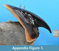 The beak was photographed in its sagittal plane using a Nikon 3200 camera with a Nikkor 60 mm micro lens (Figure A1). Digitizing follows that of Clark et al. (2015) and Aldridge (2009). Four reference points as a square on a steel ruler gave a standard deviation of 0.008 mm (i.e. ± 0.016 mm) for coordinate values. Image resolution was 42 pixels per mm. 392 outline points were digitized along the hood, from the beak’s rostral tip to the hood extremity. These outline points are provided as the data frame exColossalSquidBeak in the supplementary R package logspiral. Maximum length of growth along the beak is 125.18 mm.
While the overall beak outline is that of a logarithmic spiral, there are undulations of accretionary growth clearly evident, more so in the hood region of the beak (see arrows in Figure A1). Manual inspection of the beak surface shows the larger undulations as having ~0.2 mm amplitude and being spaced between ~ 10 to ~20 mm apart. However, undulations near the rostral tip are difficult to discern by eye, which is where spiral fitting should prove especially useful.
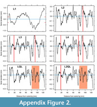 Following the steps of Appendix 2, the outline was first interpolated to provide 600 equally spaced points from the rostral tip. The L1 fit to the upper beak was not a close fit, with spiral deviations having a 1.5 mm range (Figure A2, top left). Comparing the deviations of this L1 fit to the catalogue suggests that transition spirals (LQL, L2QL) and abrupt change spirals (L3, L4) be considered for this upper squid beak. All code for the above and the following steps is provided with documentation of this beak’s outline data in logspiral.
Fitting a spiral with one abrupt change results in a dramatic reduction in overall spiral deviations exposing the undulations or cycles in growth (Figure A2 top right). However, the change location is also where there is a 0.5mm range in spiral deviations, something not seen on the actual beak. As noted in the main text above, coincidence of extreme spiral deviations at or near an abrupt change suggests a transitional logarithmic spiral for accretionary growth. Fitting L3 and L4 spirals still retains the single 0.5 mm peak at the abrupt change (Figure A2, middle row). However, fitting a transition spiral converts the single peak to two peaks of ~ 0.2 mm amplitude consistent with what is seen on the beak (Figure A2, bottom row).
 The fit that provides the least variation in spiral deviations is that of a L2QL spiral. The center of spiral transition occurs 92mm along the hood from the rostral tip, with a possible abrupt change located 18mm from the rostral tip. This beak has an initial spiral angle of 30 degrees, with an angle of 25 degrees after the transition. In contrast, many of brachiopods studied so far have larger spiral angles that typically increase after an adult change in shape, which may reflect constraints of valve articulation, occluded growing margins, and bonded substrate, none of which apply in squid beaks.
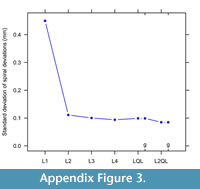
A scree plot of variation in spiral fits displays the L2QL choice (Figure A3). Having a generalized or non quadratic transition barely changes the spiral deviations. Also, final choice is determined by spiral deviations matching the magnitude of undulations or cycles in growth and lowest standard deviation (Figure A3).
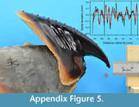
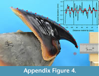 Wavelet decomposition of the L2QL spiral deviations discloses three scales of variation that explain 80% of the changes in Figure A2, bottom right. The 26 wavelet scale contributes 20% variation, and reconstruction highlights seven, possibly eight growth cycles (Figure A4). When combined with the next highest scale (to a total 60% of variation explained) wavelet reconstruction produces nine cycles matching the observed undulations on the upper beak (Figure A5). Adding the third wavelet scale represents additional changes of ~ 0.02mm in spiral deviations, or ~1-2 pixels in the image digitized, which is the same as the measurement limits for the photograph. Hence only two wavelet scales (26 and 25) are considered as having biological meaning while the third as being noise in this beak outline. Cycles are relatively regular, and in the absence of any other results, are conjectured as being linked to annual diet and temperature changes or spawning events.
 While the above results apply to only one squid, they do suggest at least two preliminary hypotheses to consider when more complete specimens are available. One is that colossal squid undergo an adult transition change in growth, the other being that colossal squid can reach an age of at least seven years.
