FIGURE 1. Right upper molar rows (M1-3) of three representative sparassodonts in occlusal view: (A) Patene coluapiensis (AMNH 28448); (B) Sipalocyon gracilis (AMNH 9254, left reversed), and (C) Cladosictis patagonica (MACN-A 5950), showing how the teeth at a certain position in the tooth row (tooth locus) in one taxon can resemble a different tooth position in another taxon (e.g., the M3 of C. patagonica resembles both the M2 of Sipalocyon gracilis and the M1 of Patene coluapiensis). Anterior is to the right in all images. Scales equal 5 mm.
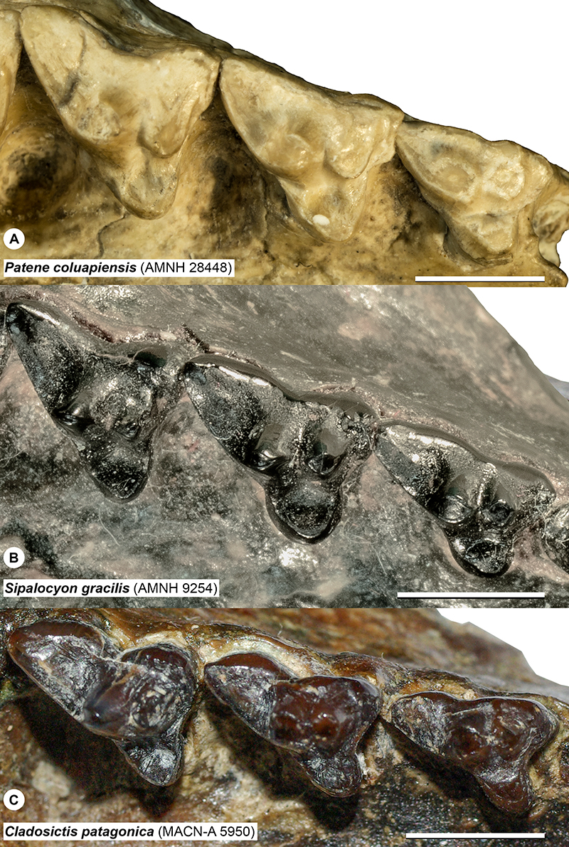
FIGURE 2. Right M2 of Acyon myctoderos (UATF-V-000926), a specimen close to the mean shape of the entire dataset, showing the morphological features of interest (A) and geometric morphometric landmarks and semilandmarks (B) used in this study. Anatomical abbreviations: alc, anterolabial cingulum (often extensive and continuous with preparaconular crista); cc, centrocrista; ef, ectoflexus; mco, metaconule; met, metacone; msl, metastylar lobe of stylar shelf; par, paracone; pco, paraconule; pmc, postmetacrista; ppc, preparacrista; pro, protocone; psl, parastylar lobe of stylar shelf; ss, stylar shelf; StA, stylar cusp A; StB, stylar cusp B. In B, squares represent fixed landmarks and circles represent semilandmarks.
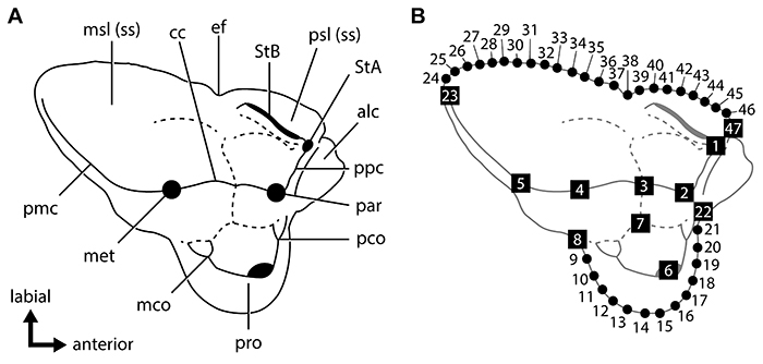
FIGURE 3. Right upper molar row of Borhyaena tuberata (MACN-A 6203), showing the change in absolute and relative sizes of the paracone and metacone from M1-3 and the relatively little inter-locus variation in stylar shelf morphology. Scale equals 5 mm.
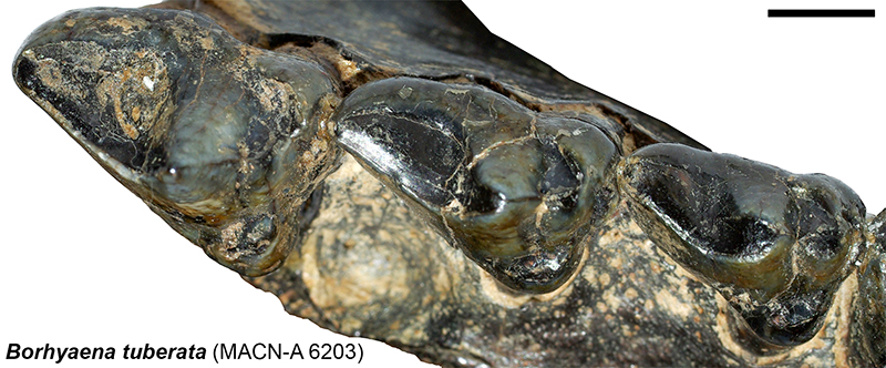
FIGURE 4. Plot of the first two principal components (PCs) of variation of the Procrustes-transformed landmark dataset for the all-taxon, trigon + talon dataset along with deformation grids representing the extreme changes in shape on each axis relative to the mean shape of the entire sample. Upper molar loci are plotted by color, with unknown specimens (M?) in black. Circled region in the upper right corner of the graph represents specimens of the Tiupampa taxa Allqokirus and Mayulestes.
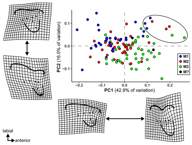
FIGURE 5. Plot of the first two principal components (PCs) of variation of the Procrustes-transformed landmark dataset for the all-taxon, trigon-only analysis along with deformation grids representing the extreme changes in shape on each axis relative to the mean shape of the entire sample. Upper molar loci are plotted by color, with unknown specimens (M?) in black.
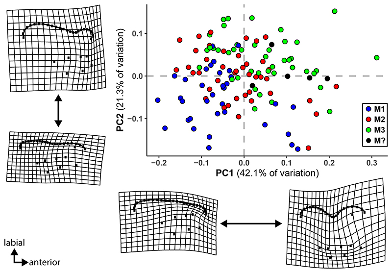
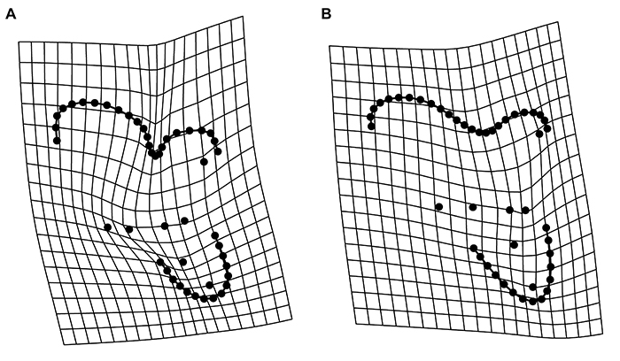
FIGURE 6. Inter-locus variation in the M1-3 of Sparassodonta as shown by the Procrustes-transformed coordinates of the geometric morphometric analysis. (A) Superimposed differences between tooth loci in the Procrustes-transformed coordinates of the average shape of M1 (large gray circles) and M3 (small black circles). The other three images show deformation grids from the average shape of all 114 examined specimens relative to the average shape of (B) M1, (C) M2, and (D) M3. Differences between loci are magnified by a factor of 3 to better illustrate patterns of variation.
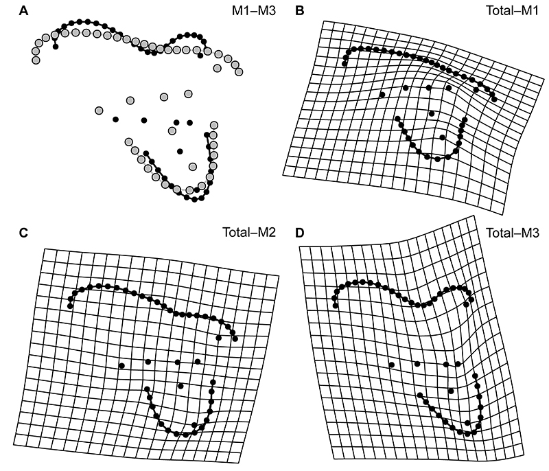
FIGURE 7. Plot of shape data (as regression score; see Drake and Klingenberg, 2008 for definition) versus natural log centroid size for all teeth of known locus in the trigon + talon dataset, showing the allometric signal in the data and the slight clustering of the teeth by locus. The extreme outlier in centroid size is the M3 of Proborhyaena gigantea, which is very large compared to the other teeth examined.
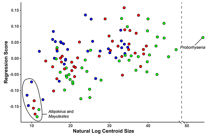
FIGURE 8. Plot of teeth by locus on the first two principal components for the all-taxon, trigon + talon dataset, color-coded as pertaining to either Borhyaenoidea, Hathliacynidae, or basal Sparassodonta.
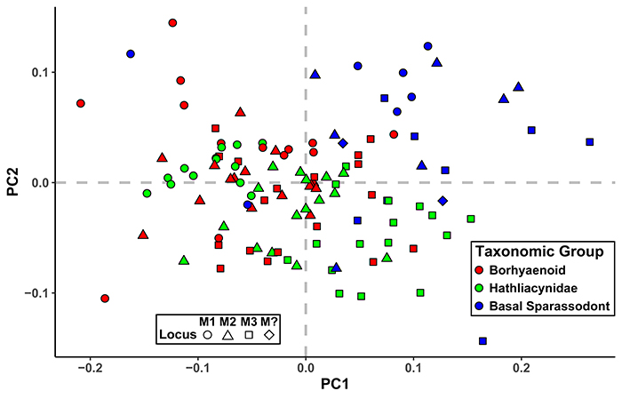
FIGURE 9. Plot of teeth by locus on the first two principal components for the all-taxon, trigon + talon dataset, color-coded by relative grinding area (RGA) for that particular taxon. Gray symbols represent taxa for which RGA could not be measured.
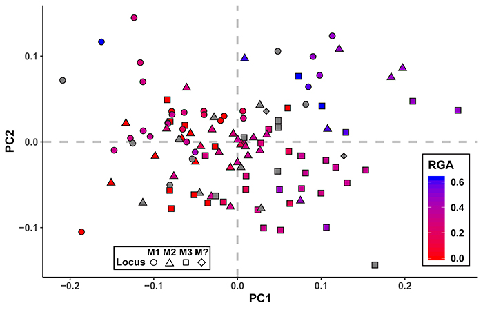
FIGURE 10. Plot of the first two canonical variates (CVs) of the all taxon, trigon + talon discriminant analysis, with tooth locus coded by symbol and incorrectly-classified specimens uncolored. Convex hulls represent morphospace occupied by each tooth locus.
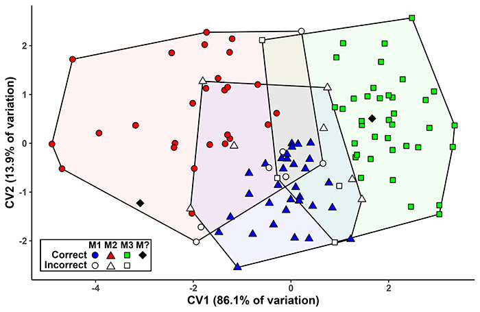
FIGURE 11. Similar to Figure 10, but with the trigon-only dataset. Plot of the first two canonical variates (CVs) of the all-taxon, trigon-only discriminant analysis with tooth locus coded by symbol and incorrectly-classified specimens uncolored. Convex hulls represent morphospace occupied by each tooth locus.
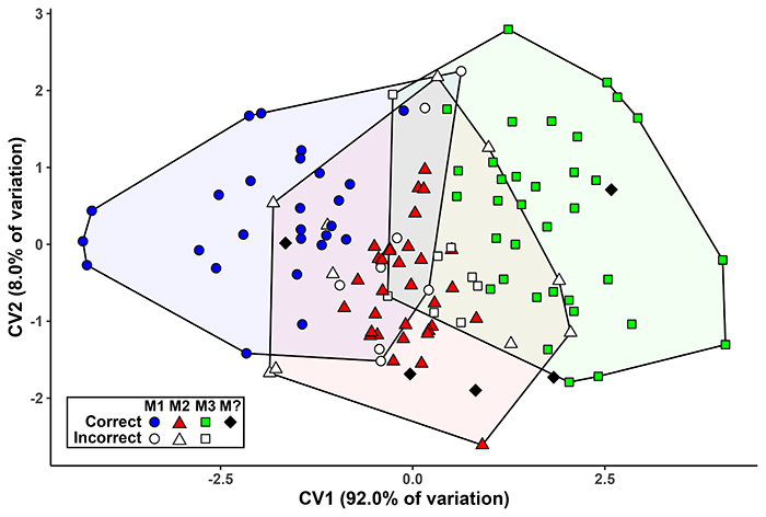
FIGURE 12. Plot of the first two canonical variates (CVs) of the reduced taxon (no Tiupampa taxa, borhyaenids, or thylacosmilids), trigon-only discriminant analysis with tooth locus coded by symbol and incorrectly-classified specimens uncolored. Convex hulls represent morphospace occupied by each tooth locus.
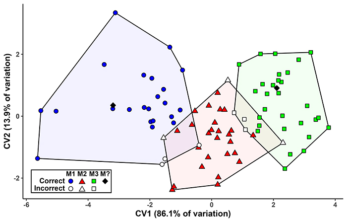
FIGURE 13. Superimposed landmark diagrams visualizing shape changes between M1 (large gray circles) and M3 (small black circles) of selected non-borhyaenid sparassodonts: (A) Allqokirus australis (MNHC 8267), (B) Patene coluapiensis (AMNH 28448), (C) Procladosictis anomala (MACN-A 10327), (D) Hondadelphys fieldsi (UCMP 37960), (E) Sipalocyon gracilis (AMNH 9254), (F) Lycopsis longirostrus (UCMP 38061), (G) Prothylacynus patagonicus (MACN-A 707), (H) Thylacosmilus atrox (MMP 1443).
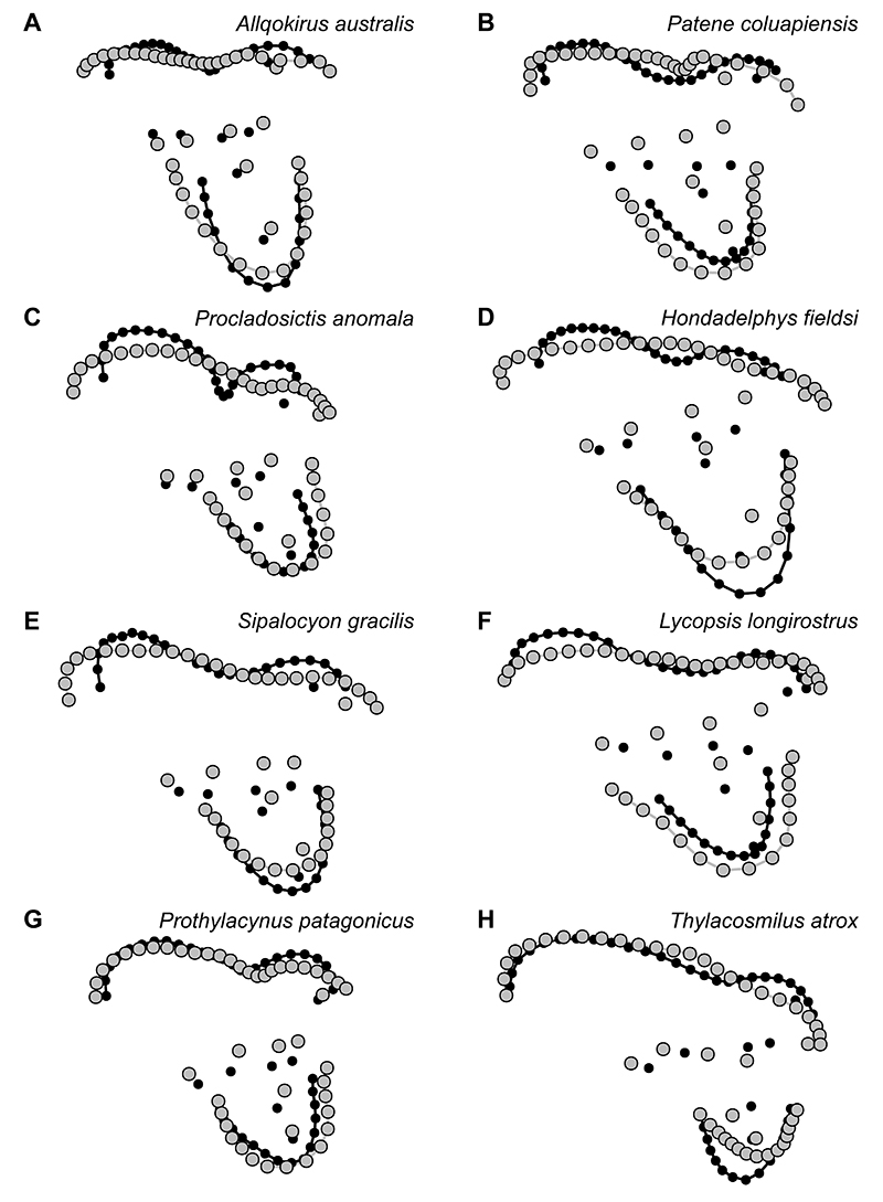
FIGURE 14. Visualization of shape changes in two Miocene borhyaenids that show little change between tooth loci. (A) M1 (gray) and M3 (black) of Borhyaena tuberata (MACN-A 6404) and (B) M2 (gray) and M3 (black) of Arctodictis sinclairi (AMNH 27909).
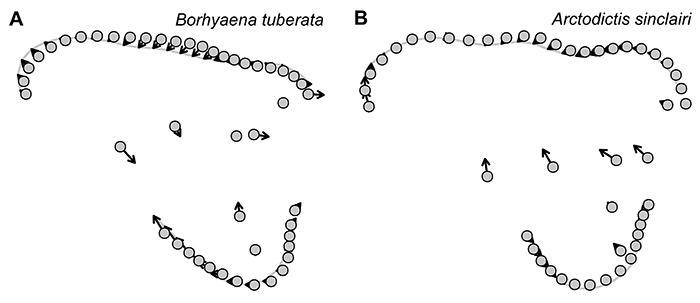
FIGURE 15. Allometric shape variation in the M1-3 of Sparassodonta as shown by the Procrustes-transformed coordinates. (A) Superimposed differences in allometric shape at the smallest (black) and largest (gray) extremes of the size range of the dataset. (B-C) Deformation grids showing differences in allometric shape variation between the sample average and (B) minimum size and (C) maximum size. Differences between loci are magnified by a factor of 2 to better illustrate patterns of variation.
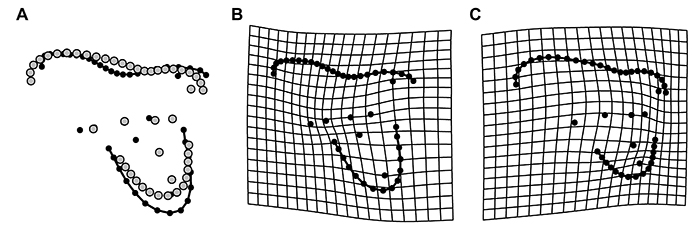
FIGURE 16. (A) TPS deformation grid showing allometric shape variation extrapolated beyond the lower bounds of the present dataset by a factor of 3 compared to (B) a photograph of the M3 of Pediomys elegans (modified from Davis, 2007: fig. 3c). Scale equals 1 mm.
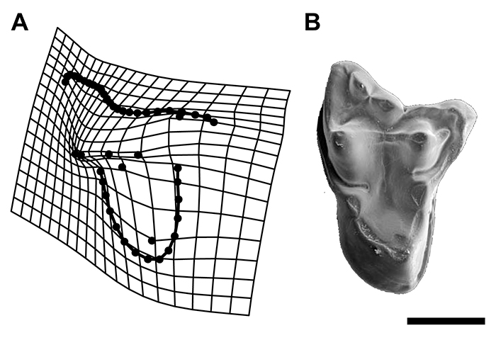
FIGURE 17. Comparison of the TPS deformation grids for the M3 of Procladosictis anomala (A) and the mean M3 shape for the entire sample exaggerated by a factor of 3 (B), both contrasted against the mean tooth shape for the entire sample.