FIGURE 1. Sample scores from detrended correspondence analysis (DCA) performed on benthic foraminiferal assemblages in the >63 µm size fraction from Integrated Ocean Drilling Program Expedition 341 Site U1419 in the Gulf of Alaska used in the simulation case study. A. DCA Axis 1 values for 355 assemblages from Sharon et al. (2021); B. DCA Axis 1 values for 47 assemblages representing a “pilot” data set of samples available and processed in 2016.
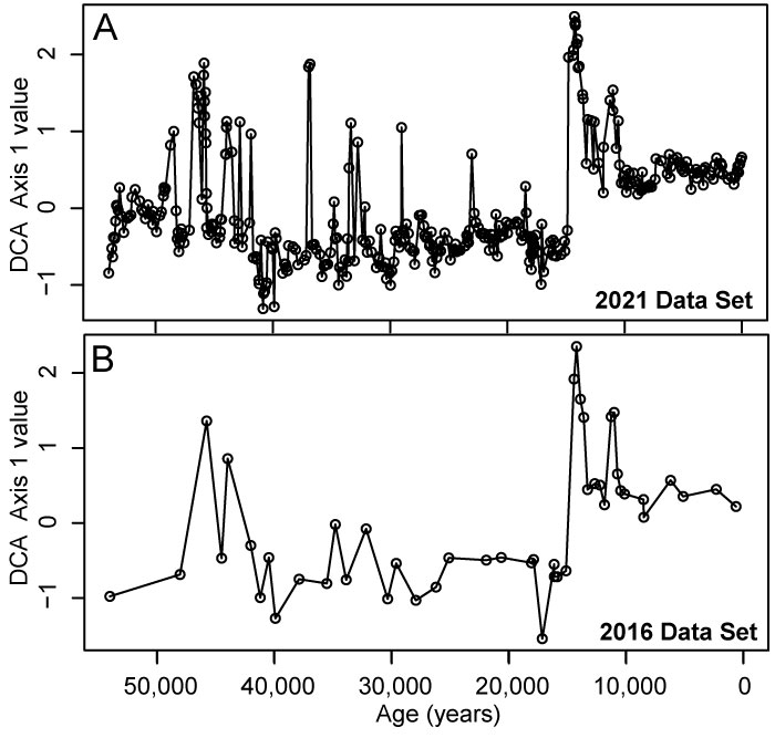
FIGURE 2. Simulation workflow in the paleontological assemblage mixer (paleoAM). A. Relative abundances of a given species (Epistominella pacifica) from the 355 samples of the 2021 data set, along the empirically derived DCA Axis 1 gradient. B. The per-bin mean of absolute abundance of E. pacifica across all samples within each bin. Absolute abundances are calculated from the relative abundances in A by rescaling the relative abundances to 10000 total specimens. C. Scaled kernel density estimates for E. pacifica, which depict the predicted abundance distribution of E. pacifica along DCA Axis 1 after fitting a kernel density estimate to the absolute abundances in B. D. Scaled kernel density estimates, like in C, for all taxa in the dataset showing their differing predicted abundance distributions along DCA Axis 1 with the kernel density of E. pacifica shown in C marked with an asterisk. E. Visual representation of parameters varied within the simulation along a vertical sediment core. From left to right: standard scenario, increased excursion magnitude, increased background value, increased resolution potential, sampling completeness, bioturbation and increased transition duration. Stacked rectangles represent potential sample intervals. In the first and last column, black dots indicate which intervals are sampled, gray dots indicate unsampled intervals. In the standard scenario, all potential sample intervals are sampled. Curved arrows denote sediment mixing among potential sample intervals.
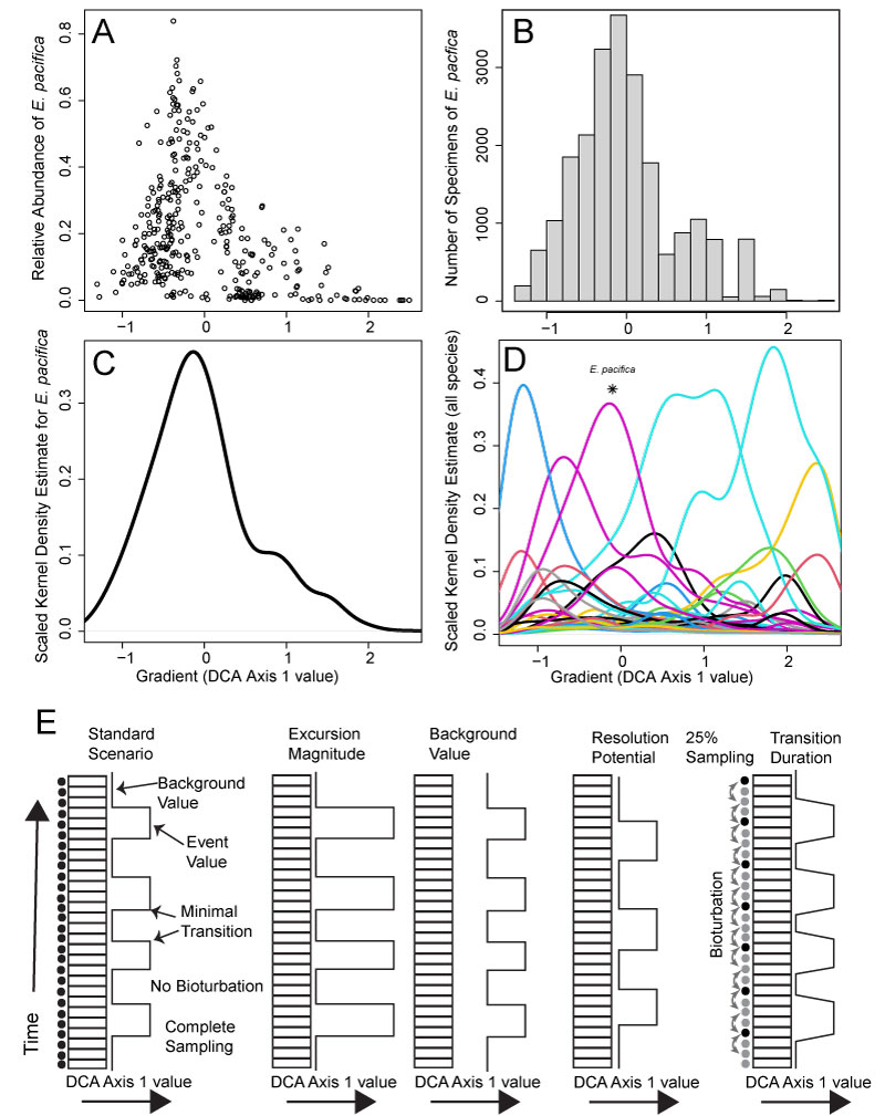
FIGURE 3. Multivariate comparison of empirical and simulated foraminiferal assemblages. A. Detrended correspondence analysis showing empirical (red filled) and simulated (black open) assemblages in the same ordination space. B. DCA1 scores for empirical samples paired with the DCA1 score of the corresponding simulated sample. Dotted line is the 1:1 line and is largely obscured by the points. C. All pairwise dissimilarities among empirical samples plotted against the average pairwise dissimilarity of 300 corresponding samples simulated at the same DCA1 values. Color scale depicts the density of dissimilarities with higher concentrations of dissimilarities in brighter colors. Black line is the 1:1 line.
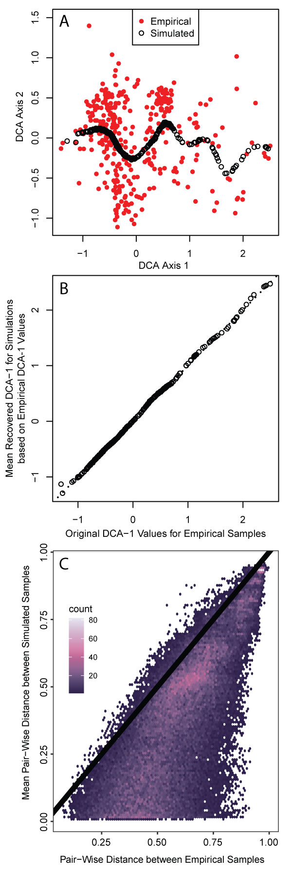
FIGURE 4. Percentage of events that are accurately detected and median excursion magnitudes for simulations performed with background DCA-1 values of -0.5, 0.5 and 1. For A and B, simulations used a background DCA-1 value of -0.5; for C and D, a background DCA-1 value of 0.5; for E and F, a background DCA-1 value of 1. Excursion magnitude (y-axis) indicates the difference between the simulated background DCA-1 value and the simulated event DCA-1 value. Resolution potential (x-axis) is the event duration divided by the time represented by the sample interval. A, C and E. Color shading indicates the percentage of events that are accurately detected by at least one sample (i.e., the sample produces a DCA-1 value outside the 95% envelope of samples simulated at the background value, and within one DCA-1 unit of the simulated excursion magnitude). B, D and F. Color shading indicates the median excursion magnitude of all samples that intersect an event. Contour lines show the parameter space where 50% (dashed line), 75% (dotted line) and 95% (solid line) of events are accurately detected.
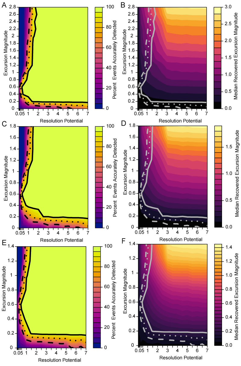
FIGURE 5. Effect of varying transition duration. Each panel represents a set of simulations generated at transition interval lengths of 0.001 times the event duration for A, 0.5 times the event duration for B, 1.0 times the event duration for C, and 5.0 times the event duration for D. Background DCA-1 value is -0.5 and completeness is 100%. Excursion magnitude (y-axis) indicates the difference between the simulated background DCA-1 value and the simulated event DCA-1 value. Resolution potential (x-axis) is the event duration divided by the time represented by the sample interval. Color shading indicates the median excursion magnitude of all samples that intersect an event. Contour lines show the parameter space where 50% (dashed line), 75% (dotted line) and 95% (solid line) of events are accurately detected.
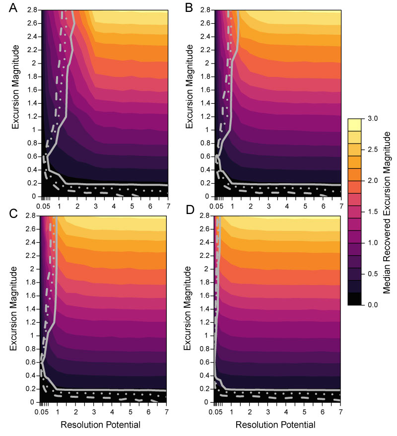
FIGURE 6. Effect of varying completeness with the duration of transition intervals. Simulation results with 25% completeness and transition lengths 0.001 times the event duration for A; and 25% completeness with transition lengths of five times the event duration for B. Background DCA-1 value is -0.5 and no bioturbation occurs. Excursion magnitude (y-axis) indicates the difference between the simulated background DCA-1 value and the simulated event DCA-1 value. Resolution potential (x-axis) is the event duration divided by the time represented by the sample interval. Color shading indicates the median excursion magnitude of all samples that intersect an event. Contour lines show the parameter space where 50% (dashed line), 75% (dotted line) and 95% (solid line) of events are accurately detected.
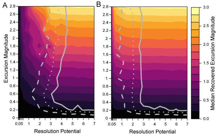
FIGURE 7. The interaction of bioturbation, completeness and transition duration. All simulations figured include bioturbation and use a background DCA-1 value of -0.5. Simulation results for 100% sampling completeness and transition durations 0.001 times the event duration for A; 100% sampling completeness and transition durations five times the event duration for B; 25% sampling completeness and transition durations 0.001 times the event duration for C; 25% sampling completeness and transition durations five times the event duration for D. Excursion magnitude (y-axis) indicates the difference between the simulated background DCA-1 value and the simulated event DCA-1 value. Resolution potential (x-axis) is the event duration divided by the time represented by the sample interval. Color shading indicates the median excursion magnitude of all samples that intersect an event. Contour lines show the parameter space where 50% (dashed line), 75% (dotted line) and 95% (solid line) of events are accurately detected.
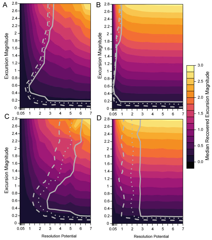
FIGURE 8. Difference maps showing the percentage of events accurately detected by simulations without bioturbation subtracted from the percentage of events accurately detected by simulations with bioturbation. 100% sampling completeness and transition durations 0.001 times the event duration for A; 100% sampling completeness and transition durations five times the event duration for B; 25% sampling completeness and transition durations 0.001 times the event duration for C; 25% sampling completeness and transition durations five times the event duration for D. The solid black line marks the contour line for zero difference between the bioturbated and non-bioturbated simulations.
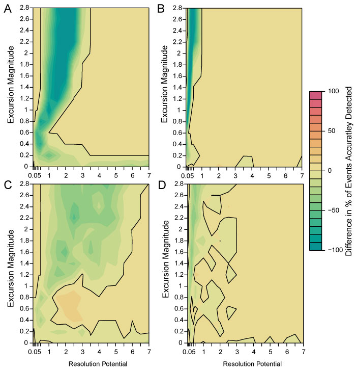
FIGURE 9. DCA-1 values observed when assemblages simulated at different event values are mixed with different proportions of the background assemblage. For A, the maximum DCA-1 value observed is shown; for B, the median DCA-1 value observed; and for C, the minimum DCA-1 value observed. In all cases, background assemblages are simulated at a DCA-1 value of -0.5 and are mixed with an event assemblage with a DCA-1 value as given on the x-axis.
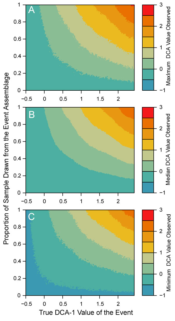
FIGURE 10. Percentage of DCA-1 values obtained from simulations that fall within a 95% envelope of three DCA-1 values: (A) 0.0 (B) 1.0 and (C) 2.0. These values were selected as example observations from a hypothetical empirical data set and are marked by a green line in each subfigure. The bounds of the 95% confidence envelope were calculated by repeatedly simulating assemblages at the indicated empirical DCA-1 value and finding the two-tailed 95% quantile on the DCA-1 values obtained from those simulated assemblages. In the mixed assemblage simulations, background assemblages are simulated at a DCA-1 value of -0.5 and are mixed with an event assemblage with a DCA-1 value as given on the horizontal axis, with the proportion of mixing indicated on the vertical axis. In all three cases, the region the target DCA-1 value is observed in the simulations is a narrow ridge in probability space.
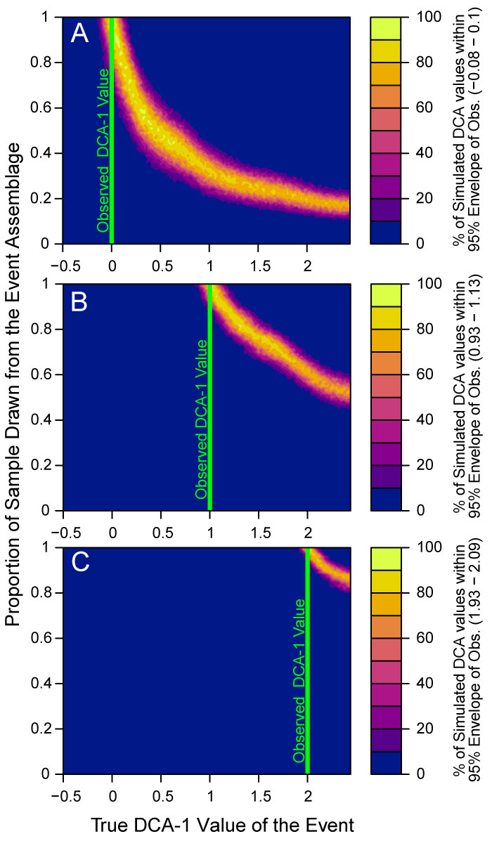
FIGURE 11. Comparison of event detection between the 2016 “pilot” data set and the final 2021 data set and three example excursion magnitudes. A and B are simulations without bioturbation, C and D are simulations with bioturbation. A and C show the percentage of events accurately detected whereas B and D show the percentage of events detected irrespective of accuracy. In all simulations, sampling completeness is 25% and the transition between background (DCA-1 value = -0.5) and events is abrupt (0.001 times the event length).
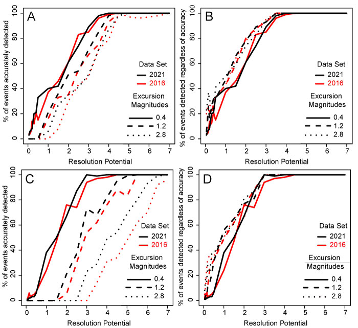
FIGURE 12. Effect of sample thickness on accurate detection of events with excursion magnitudes of 2.8 DCA-1 units. Y-axis shows the percentage of accurately detected events at different sedimentation rates (x-axis) for three different event durations: 50 years, 100 years and 1000 years. Simulations are for the 2016 data set to approximate how a researcher might use a pilot data set to design a sampling procedure and are based on sampling with 25% completeness. A is simulations without the effect of bioturbation; B is simulations with the effect of bioturbation.
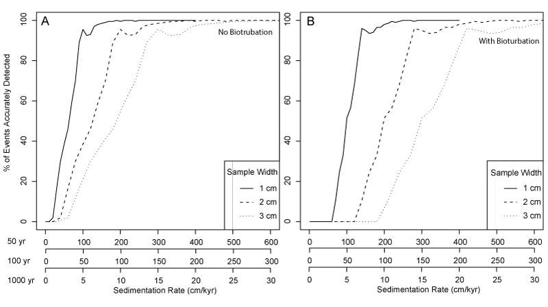
FIGURE 13. Resolution potential of the GoA record for 100-year long events. Resolution potential is calculated assuming 3 cm-thick samples, with estimates of sedimentation rates in 500-year intervals from Walczak et al. (2020). Dotted red line shows the resolution potential at which 95% of simulated assemblages accurately detect extreme events (excursion magnitude = 2.8 DCA-1 units) when bioturbation is present and sampling completeness is 100%. Dashed blue line is similar but for simulations at 25% sampling completeness.
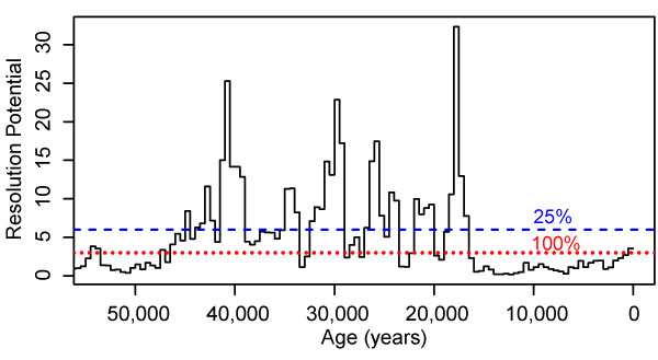
FIGURE 14. Estimated ability of the record to detect 100 year-long events with 3 cm samples, given a known sedimentation rate at three excursion magnitudes (0.4, 1.2 and 2.8), based on ‘worst-case scenario’ simulations with 25% sampling, bioturbation, rapid transitions between events and the background condition (-0.5 DCA-1 value). A and B are simulated with an excursion magnitude of 0.4; C and D are simulated with an excursion magnitude of 1.2; and E and F are simulated with an excursion magnitude of 2.8. A, C and E show the percentage of events that are detectable above a background value of -0.5. An event is detected if a sample has an observed DCA-1 value exceeding the 95% quantile of the DCA-1 value of assemblages simulated at the background value. B, D and F show the median DCA-1 values recovered from samples intersecting simulated events. Values that fall above the blue dashed line are detected; that is, they exceed the 95% quantile of the DCA-1 value of assemblages simulated at the background value. Values that fall above the red dotted line are accurately detected; that is, they exceed the 2.75% quantile on DCA-1 values recovered from simulations at the event value.