FIGURE 1. Trilobite generalised moult configurations featuring in the dataset presented here. A: Olenus truncatus Brünnich, 1781, PMU unnumbered specimen, cephalic sutures configuration group, B: Ellipsocephalus sp. Zenker, 1833, PMU 28642, Salter’s configuration, C: Trimerocephalus mastophthalmus Richter, 1856, NHMUK I.5100, Salter’s configuration, D: Dalmanitina socialis (Barrande, 1846), NHMUK 42341, Zombie configuration, E: Paradoxides gracilis Boeck, 1827, NHMUK 42440, Henningsmoen’s configuration, F: Estaingia bilobata Pocock, 1964, SAM-P 46956, Henningsmoen’s configuration, G: Estaingia bilobata, SAM-P 43767, cephalic sutures configuration group, H: Redlichia takooensis Lu, 1950, SAM-P 43593, Salter’s configuration, I: Accadoparadoxides pinus Westergård, 1936, PMU 25995, cephalic sutures + inversion configuration group, J: Phillipsia sp. Portlock, 1843, NHMUK I.1092, cephalic sutures + inversion configuration group. Scale bars equal 5 mm for A, B, F, G, J; 10 mm for C-E, H, I.
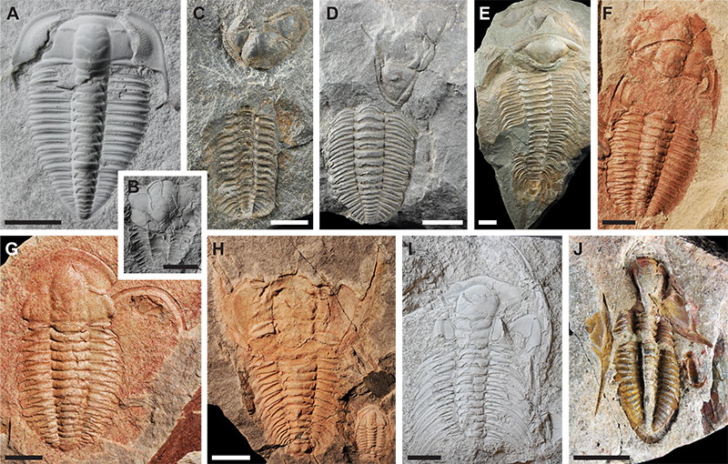
FIGURE 2. Illustration of measurements taken on trilobite specimens, where possible given specimen preservation, shown on simplified drawing of Cryphoproetus. CrW: cranidial width (tr.), CrL: cranidial axial length (sag.), CThW: cephalothoracic joint width (tr.), ThW: thoracic maximum width (tr.), ThL: thoracic axial length (sag.), PyW: pygidial maximum width (tr.), PyL: pygidial axial length (sag.), TBL: total axial body length (sag.).
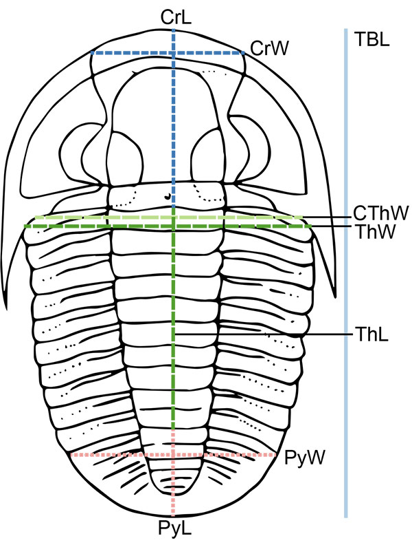
FIGURE 3. Principal Components Analysis plots with specimens grouped by mode of moulting (A) or generalised moult configuration (B) (see legends). Plot C shows the contributions of the dataset variables to the morphospace in A and B; directionality of each arrow represents how it varies across the morphospace, and length of each arrow represents its comparable impact on the morphospace. TT: thoracic tergite number, LT: thoracic axial length, WT: thoracic maximum width, CW: cranidial width, CL: cranidial axial length, CJW: cephalothoracic joint width.
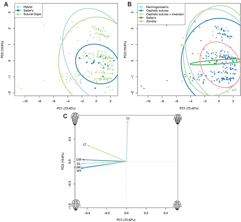
FIGURE 4. NMDS analysis plots with specimens grouped by mode of moulting (A) or generalised moult configuration (B) (see legends).
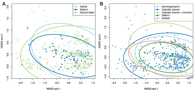
FIGURE 5. Box plots displaying mean (black square) and median (horizontal black line) average thoracic tergite number for each mode of moulting group (A) and generalised moult configuration (B). Grey jitter shows the plotted points comprising the boxes (jitter spread across the x-axis is purely for visualisation), and black points show suggested outliers.
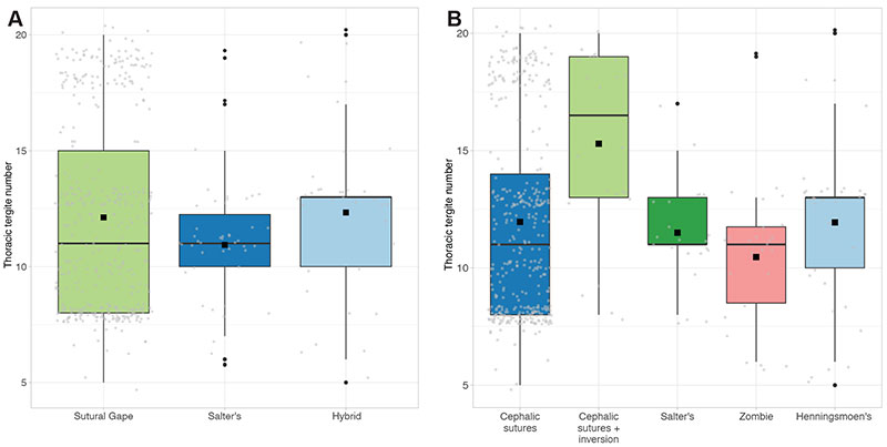
FIGURE 6. Scatterplots of the total dataset, for each metric morphometry variable. Data is grouped by mode of moulting (see legend). Linear regression lines represent the MANCOVA analysis models (see text).
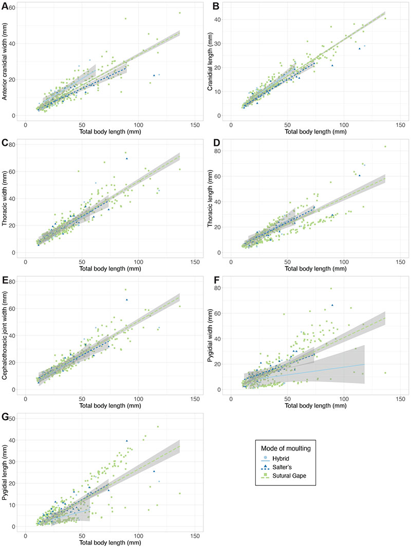
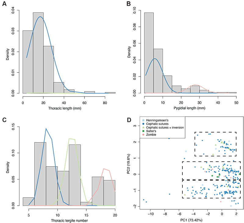
FIGURE 7. Histograms of notable variables within the dataset (using only complete data entries), with plotted EM algorithm-calculated distributions. A: thoracic axial length histogram, with two estimated distributions. B: pygidial axial length histogram, with three estimated distributions; two (blue and green lines) are exactly overlapping, indicating they represent the same distribution. C: thoracic tergite number, with three estimated distributions. D: PCA plot, with specimens grouped by generalised moult configuration (see legend) and ellipses removed (original plot in Figure 3B); dashed black boxes roughly demonstrate the three major data clusters apparent in the morphospace.