

Article Search
Volume 27.1
January–April 2024
Full table of contents
ISSN: 1094-8074, web version;
1935-3952, print version
Recent Research Articles
See all articles in 27.1 January-April 2024
See all articles in 26.3 September-December 2023
See all articles in 26.2 May-August 2023
See all articles in 26.1 January-April 2023
APPENDIX
Program listings
Download archive with Fortran listings and executable applications for PC: 278_listing.zip (Expand by double-clicking on the archive icon und then by using the extract command in WinZip 11.1).
Fortran programming originally performed using Fortran 77 from Absoft for Macintosh computers (MPW), and then translated to the Windows environment using the free distribution software Force 2.0 fortran compiler and editor developed by Luiz Lepsch Guedes, which is available from the URL http://force.lepsch.com.
Subdirectory [Grid2]:
Subdirectory [Example]:
Tutorial for Gridd_winversion2.exe
Application Gridd_winversion2.exe for PCs.
"List_of_files.txt": Containins the names of input files with bivariate X,Y measurements.
"Inputxxxxxxxxxx1.txt" and "Inputxxxxxxxxxx2.txt" are two examples with bivariate X,Y measurements for C. leptoporus.
Subdirectory [Force_listing]:
Gridd_winversion2 (Force 2.0 source file)
Listing_Gridd_winversion2.txt
Subdirectory [Grid_toVox3/Gmenardi]:
Subdirectory [Example]:
Application Grid_to_Vox3_win.exe for PC's.
Tutorial for Grid_to_Vox3_win.exe
"List_of_files.txt": Containins the ages and names of input files with gridded matrices.
"input1xxxxxxxxxx_grd" and "input2xxxxxxxxxx_grd" are two examples with frequency matrices.
Subdirectory [Force_listing]:
Grid_to_Vox3_win (Force 2.0 source file)
Listing_Grid_to_Vox3_win.txt
Subdirectory [Grid_toVox4/Cleptoporus]:
Subdirectory [Example ME69-196]:
Application Grid_to_Vox4_win.exe for PC's.
Tutorial for Grid_to_Vox4_win.exe
"List_of_files.txt": Containins the ages and names of input files with gridded matrices.
The files
"002-003cmxxxxxxx_grd"
"033-034cmxxxxxxx_grd"
"246-247cmxxxxxxx_grd"
"285-287cmxxxxxxx_grd"
"471-472cmxxxxxxx_grd"
are examples with frequency matrices for C. leptoporus.
Subdirectory [Force_listing]:
Grid_to_Vox4_win (Force 2.0 source file)
Listing_Grid_to_Vox4_win.txt
More detailed explanations Grid_to_Vox applications
Data sets
(Expand by double-clicking on the archive icon und then by using the extract command in WinZip 11.1).
Explanations for the C. leptoporus data-set, in subdirectory [CLEPTOP]:
Subdirectory [MEASURES/DIAM_EL] contains the original bivariate measurements of coccolith diameter (in µm) versus the number of elements, separated by a comma. Each file represents a sample. The data are sorted into core locations. Holocene surface sediment samples are sorted into folder [HOLOCENE]. For the provenance of Holocene materials refer to Knappertsbusch et al. (1997), for the provenances and ages of the remaining material refer to Knappertsbusch (2000). Open files with MS Word to watch the formatting.
Subdirectory [GRIDDED] contains absolute frequencies (number of coccoliths per grid-cell) per sample per core using a grid-cell size of 1µm in length and 2 elements in width. The gridded data for C. leptoporus were calculated using program Grid2 from the binary measurements of diameter versus number of elements in the distal shield in each sample and are from Knappertsbusch (2000). Open files with MS Word to watch the formatting.
Subdirectory [INP_VOX] contains the coccolith frequency data (ALL_XYZFsn) arranged by core after application of the Grid_toVox4 program was performed. File ALL_XYZFsn can be directly imported to Voxler. X denotes the diameter in µm, Y the number of elements in the distal shield, and Z indicates the coccolith frequency per grid-cell. During running of Program Grid_to_Vox4, the options "with scaling of axes and with normalization of Frequency (option 1)" and "output to one single file (option 1)" were applied. The common age to all cores (ZMAX) was 23.08 Ma.
The lowercase letter "s" of the filename ALL_XYZFsn indicates, that all axes were standardized to units between 0 and 1, whereas the lowercase letter "n" indicates, that the coccolith frequencies were normalized by conversion from absolute to relative frequencies. Open files with MS Word to watch the formatting.
The MS Word file "statistics" in folder [AGES] reproduces a survey of samples, numerical ages, and statistical data for all C. leptoporus data, as they were published in Knappertsbusch (2000) and used in the present study for construction of volume density plots.
Explanations for the G. menardii data-set, in subdirectory [GMENAR]:
Subdirectory [MEASURES] contains the split-weighted morphometric measurements of G. menardii from DSDP Sites 502A and 503A, arranged per sample (see Knappertsbusch, 2007). In "composed_files" all measurements are merged together into one single file. The format of the header line of "composed_files" applies also to the individual sample files. For collecting bivariate measurements of spiral height versus axial length cited in the paper, the respective columns (X,Y) must be extracted before they can be fed to the gridding program. Open files with MS Word or MS Excel to watch the formatting.
Subdirectory [GRIDDED] contains absolute frequencies (number specimens per grid-cell) per sample for the DSDP Sites 502 and 503. Also for these data program Grid2 was applied to bivariate measurements of X (spiral height, in µm) versus Y (axial length, in µm) using a grid-cell size of 100 µm in length and 50 µm in width as was discussed in Knappertsbusch (2007). The subdirectory [XY data] provides the bivariate measurements of X versus Y for each sample; the filenames encode for the absolute age (in million years), the ages were taken from the study of Knappertsbusch (2007). Open files with MS Word or MS Excel to watch the formatting.
Subdirectory [INP_VOX] contains the files "ALL_XYZFsn_ZMAX=8Ma", that were obtained with
Grid_to_Vox3 on the respective lists of gridded data files from DSDP Sites 502 and 503.
Open files with MS Word or MS Excel to watch the formatting.
Parameters for Gridding in Grid2.2:
Data range: 0-700µm, 0-1600µm,
Grid-cell size: DeltaX = 50µm, DeltaY = 100µm.
The files ALL_XYZFsn_ZMAX=8Ma (same name for DSDP Sites 502 and 503) can directly be imported to the spreadsheet from Voxler.
Parameters set in Program Grid_to_Vox3:
Option "with scaling of axes and with normalization of Frequency" (Option 1)
Option "output to one single file (option 1)"
In file "ALL_XYZFsn_ZMAX=8Ma" the axes were standardized to units ranging from 0 to 1 (indicated by the lowercase letter "s" in the filename) and frequencies F of specimens per grid-cell are normalized to relative values ranging from 0 to 100% (indicated by the lowercase letter "n" in the filename) in order to maintain inter-sample comparison.
The common age to all cores (ZMAX) was set to 8.0 Ma.
Tutorial – Program Grid_to_Vox
Given are bivariate (X,Y) scatter data from a series of samples at different geological ages. Using program Grid2.2.out discrete bivariate frequency distributions Delta X, Delta Y,Z,F are generated, with Delta X and Delta Y being the grid-cell sizes of the X- and Y coordinate axes, respectively, with Z being the geological age of a particular sample, and with F being the bivariate frequency of points per grid-cell (see, for example, Knappertsbusch, 2000). The program Grid_to_Vox3 is reserved for handling the G. menardii data set, while Grid_to_Vox4 is reserved for the C. leptoporus data set (this separation into two programs was done in order to keep computer programs as simple as possible).
Input to Grid_to_Vox:
Both Grid_to_Vox versions work in batch operating mode, so that a large number of gridded input files can be processed one after the other. Two types of input files are required: First, one text file called List_of_files, which contains a list of the age (in Ma) of the sample and the corresponding name of the file with the gridded data matrix per sample. The gridded data matrix contains the frequency distribution of the bivariate set of measurements. The age must be written in digits of five characters, followed by a comma, followed by the name of the gridded input matrix. The name of the gidded input data is 16 characters long. The second type of input files are the files with the gridded data matrices (one file per sample). The gridded data matrices need to be unformatted, i.e., without any header or column information (these must first be removed by manual editing).
Example for Grid_to_Vox3 (Globorotalia menardii):
File List_of_files:
00.340,input1xxxxxxxxxx_grd.txt
56.781,input2xxxxxxxxxx_grd.txt
Gridded data matrix (for Globorotalia menardii):
A 14x16 matrix (14 columns, 16 rows).
Delta X goes in horizontal direction (mid-points at 25, 75, 125,..., 675 micrometers).
[Intervals of Delta X=50micrometers].
Delta Y goes in vertical direction (mid-points at 50, 150, 250,...,1550 micrometers).
[Intervals of Delta Y=100 micrometers].
File input1xxxxx_grid:
1 2 3 4 5 6 7 8 9 10 11 12 13 14
15 16 17 18 19 20 21 22 23 24 25 26 27 28
29 30 31 32 33 34 35 36 37 38 39 40 41 42
43 44 45 46 47 48 49 50 51 52 53 54 55 56
57 58 59 60 61 62 63 64 65 66 67 68 69 70
71 72 73 74 75 76 77 78 79 80 81 82 83 84
85 86 87 88 89 90 91 92 93 94 95 96 97 98
99 100 101 102 103 104 105 106 107 108 109 110 111 112
113 114 115 116 117 118 119 120 121 122 123 124 125 126
127 128 129 130 131 132 133 134 135 136 137 138 139 140
140 141 142 143 144 145 146 147 148 149 150 151 152 153
154 155 156 157 158 159 160 161 162 163 164 165 166 167
167 168 169 170 171 172 173 174 175 176 177 178 179 180
181 182 183 184 185 186 187 188 189 190 191 192 193 194
195 196 197 198 199 200 201 202 203 204 205 206 207 208
209 210 211 212 213 214 215 216 217 218 219 220 221 222
Output
The format of the output data, which can be imported in Voxler is
Delta X, Delta Y, Age (Ma), Frequency
Example for file input1xxxxx_grid:
25. 50. .34 1.
25. 150. .34 15.
25. 250. .34 29.
25. 350. .34 43.
25. 450. .34 57.
25. 550. .34 71.
25. 650. .34 85.
25. 750. .34 99.
25. 850. .34 113.
25. 950. .34 127.
25. 1050. .34 140.
25. 1150. .34 154.
25. 1250. .34 167.
25. 1350. .34 181.
25. 1450. .34 195.
25. 1550. .34 209.
75. 50. .34 2.
75. 150. .34 16.
75. 250. .34 30.
75. 350. .34 44.
75. 450. .34 58.
75. 550. .34 72.
75. 650. .34 86.
75. 750. .34 100.
75. 850. .34 114.
75. 950. .34 128.
75. 1050. .34 141.
75. 1150. .34 155.
75. 1250. .34 168.
75. 1350. .34 182.
75. 1450. .34 196.
75. 1550. .34 210.
125. 50. .34 3.
125. 150. .34 17.
125. 250. .34 31.
125. 350. .34 45.
125. 450. .34 59.
125. 550. .34 73.
125. 650. .34 87.
125. 750. .34 101.
125. 850. .34 115.
125. 950. .34 129.
125. 1050. .34 142.
125. 1150. .34 156.
125. 1250. .34 169.
125. 1350. .34 183.
125. 1450. .34 197.
125. 1550. .34 211.
175. 50. .34 4.
175. 150. .34 18.
175. 250. .34 32.
175. 350. .34 46.
175. 450. .34 60.
175. 550. .34 74.
175. 650. .34 88.
175. 750. .34 102.
175. 850. .34 116.
175. 950. .34 130.
175. 1050. .34 143.
175. 1150. .34 157.
175. 1250. .34 170.
175. 1350. .34 184.
175. 1450. .34 198.
175. 1550. .34 212.
225. 50. .34 5.
225. 150. .34 19.
225. 250. .34 33.
225. 350. .34 47.
225. 450. .34 61.
225. 550. .34 75.
225. 650. .34 89.
225. 750. .34 103.
225. 850. .34 117.
225. 950. .34 131.
225. 1050. .34 144.
225. 1150. .34 158.
225. 1250. .34 171.
225. 1350. .34 185.
225. 1450. .34 199.
225. 1550. .34 213.
275. 50. .34 6.
275. 150. .34 20.
275. 250. .34 34.
275. 350. .34 48.
275. 450. .34 62.
275. 550. .34 76.
275. 650. .34 90.
275. 750. .34 104.
275. 850. .34 118.
275. 950. .34 132.
275. 1050. .34 145.
275. 1150. .34 159.
275. 1250. .34 172.
275. 1350. .34 186.
275. 1450. .34 200.
275. 1550. .34 214.
325. 50. .34 7.
325. 150. .34 21.
325. 250. .34 35.
325. 350. .34 49.
325. 450. .34 63.
325. 550. .34 77.
325. 650. .34 91.
325. 750. .34 105.
325. 850. .34 119.
325. 950. .34 133.
325. 1050. .34 146.
325. 1150. .34 160.
325. 1250. .34 173.
325. 1350. .34 187.
325. 1450. .34 201.
325. 1550. .34 215.
375. 50. .34 8.
375. 150. .34 22.
375. 250. .34 36.
375. 350. .34 50.
375. 450. .34 64.
375. 550. .34 78.
375. 650. .34 92.
375. 750. .34 106.
375. 850. .34 120.
375. 950. .34 134.
375. 1050. .34 147.
375. 1150. .34 161.
375. 1250. .34 174.
375. 1350. .34 188.
375. 1450. .34 202.
375. 1550. .34 216.
425. 50. .34 9.
425. 150. .34 23.
425. 250. .34 37.
425. 350. .34 51.
425. 450. .34 65.
425. 550. .34 79.
425. 650. .34 93.
425. 750. .34 107.
425. 850. .34 121.
425. 950. .34 135.
425. 1050. .34 148.
425. 1150. .34 162.
425. 1250. .34 175.
425. 1350. .34 189.
425. 1450. .34 203.
425. 1550. .34 217.
475. 50. .34 10.
475. 150. .34 24.
475. 250. .34 38.
475. 350. .34 52.
475. 450. .34 66.
475. 550. .34 80.
475. 650. .34 94.
475. 750. .34 108.
475. 850. .34 122.
475. 950. .34 136.
475. 1050. .34 149.
475. 1150. .34 163.
475. 1250. .34 176.
475. 1350. .34 190.
475. 1450. .34 204.
475. 1550. .34 218.
525. 50. .34 11.
525. 150. .34 25.
525. 250. .34 39.
525. 350. .34 53.
525. 450. .34 67.
525. 550. .34 81.
525. 650. .34 95.
525. 750. .34 109.
525. 850. .34 123.
525. 950. .34 137.
525. 1050. .34 150.
525. 1150. .34 164.
525. 1250. .34 177.
525. 1350. .34 191.
525. 1450. .34 205.
525. 1550. .34 219.
575. 50. .34 12.
575. 150. .34 26.
575. 250. .34 40.
575. 350. .34 54.
575. 450. .34 68.
575. 550. .34 82.
575. 650. .34 96.
575. 750. .34 110.
575. 850. .34 124.
575. 950. .34 138.
575. 1050. .34 151.
575. 1150. .34 165.
575. 1250. .34 178.
575. 1350. .34 192.
575. 1450. .34 206.
575. 1550. .34 220.
625. 50. .34 13.
625. 150. .34 27.
625. 250. .34 41.
625. 350. .34 55.
625. 450. .34 69.
625. 550. .34 83.
625. 650. .34 97.
625. 750. .34 111.
625. 850. .34 125.
625. 950. .34 139.
625. 1050. .34 152.
625. 1150. .34 166.
625. 1250. .34 179.
625. 1350. .34 193.
625. 1450. .34 207.
625. 1550. .34 221.
675. 50. .34 14.
675. 150. .34 28.
675. 250. .34 42.
675. 350. .34 56.
675. 450. .34 70.
675. 550. .34 84.
675. 650. .34 98.
675. 750. .34 112.
675. 850. .34 126.
675. 950. .34 140.
675. 1050. .34 153.
675. 1150. .34 167.
675. 1250. .34 180.
675. 1350. .34 194.
675. 1450. .34 208.
675. 1550. .34 222.
TABLE 1.Output Grid_to_Vox4 applied on sample DSDP 251A-12-1, 88cm for C. leptoporus. Values are coccolith frequencies per grid-cell. Dameter classes of 1 micrometer (from 0 through 14) are arranged horizontally, classes of two elements (from 0 through 54) are arranged vertically.
DSDP 251A-12-1, 88cm
6 t :XY->XYZ Gridded Data - Contour Plot V.1.0
27 2 14 1 .5 1
|
|
0-1 µm |
1-2 µm |
2-3 µm |
3-4 µm |
4-5 µm |
5-6 µm |
6-7 µm |
7-8 µm |
8-9 µm |
9-10 µm |
10-11 µm |
11-12 µm |
12-13 µm |
13-14 µm |
|
0-2 Elements |
0 |
0 |
0 |
0 |
0 |
0 |
0 |
0 |
0 |
0 |
0 |
0 |
0 |
0 |
|
2-4 Elements |
0 |
0 |
0 |
0 |
0 |
0 |
0 |
0 |
0 |
0 |
0 |
0 |
0 |
0 |
|
4-6 Elements |
0 |
0 |
0 |
0 |
0 |
0 |
0 |
0 |
0 |
0 |
0 |
0 |
0 |
0 |
|
6-8 Elements |
0 |
0 |
0 |
0 |
0 |
0 |
0 |
0 |
0 |
0 |
0 |
0 |
0 |
0 |
|
8-10 Elements |
0 |
0 |
0 |
0 |
0 |
0 |
0 |
0 |
0 |
0 |
0 |
0 |
0 |
0 |
|
10-12 Elements |
0 |
0 |
0 |
0 |
0 |
0 |
0 |
0 |
0 |
0 |
0 |
0 |
0 |
0 |
|
12-14 Elements |
0 |
0 |
0 |
0 |
0 |
0 |
0 |
0 |
0 |
0 |
0 |
0 |
0 |
0 |
|
14-16 Elements |
0 |
0 |
0 |
0 |
0 |
0 |
0 |
0 |
0 |
0 |
0 |
0 |
0 |
0 |
|
16-18 Elements |
0 |
0 |
0 |
0 |
0 |
3 |
0 |
0 |
0 |
0 |
0 |
0 |
0 |
0 |
|
18-20 Elements |
0 |
0 |
0 |
0 |
2 |
3 |
0 |
0 |
0 |
0 |
0 |
0 |
0 |
0 |
|
20-22 Elements |
0 |
0 |
0 |
0 |
2 |
1 |
2 |
2 |
0 |
0 |
0 |
0 |
0 |
0 |
|
22-24 Elements |
0 |
0 |
0 |
0 |
1 |
2 |
3 |
2 |
3 |
0 |
0 |
0 |
0 |
0 |
|
24-26 Elements |
0 |
0 |
0 |
0 |
0 |
1 |
4 |
4 |
12 |
3 |
2 |
0 |
0 |
0 |
|
26-28 Elements |
0 |
0 |
0 |
0 |
0 |
0 |
6 |
11 |
8 |
6 |
5 |
0 |
0 |
1 |
|
28-30 Elements |
0 |
0 |
0 |
0 |
0 |
0 |
3 |
12 |
6 |
3 |
11 |
2 |
1 |
0 |
|
30-32 Elements |
0 |
0 |
0 |
0 |
0 |
1 |
3 |
8 |
4 |
3 |
5 |
2 |
0 |
0 |
|
32-34 Elements |
0 |
0 |
0 |
0 |
0 |
0 |
3 |
2 |
2 |
1 |
0 |
0 |
1 |
0 |
|
34-36 Elements |
0 |
0 |
0 |
0 |
0 |
0 |
0 |
0 |
0 |
1 |
1 |
0 |
0 |
0 |
|
36-38 Elements |
0 |
0 |
0 |
0 |
0 |
0 |
0 |
0 |
0 |
0 |
0 |
0 |
0 |
0 |
|
38-40 Elements |
0 |
0 |
0 |
0 |
0 |
0 |
0 |
1 |
0 |
0 |
0 |
1 |
0 |
0 |
|
40-42 Elements |
0 |
0 |
0 |
0 |
0 |
0 |
0 |
0 |
0 |
0 |
0 |
1 |
0 |
0 |
|
42-44 Elements |
0 |
0 |
0 |
0 |
0 |
0 |
0 |
1 |
0 |
0 |
2 |
4 |
2 |
0 |
|
44-46 Elements |
0 |
0 |
0 |
0 |
0 |
0 |
0 |
0 |
0 |
0 |
4 |
1 |
0 |
0 |
|
46-48 Elements |
0 |
0 |
0 |
0 |
0 |
0 |
0 |
0 |
0 |
0 |
1 |
7 |
0 |
0 |
|
48-50 Elements |
0 |
0 |
0 |
0 |
0 |
0 |
0 |
0 |
0 |
0 |
0 |
0 |
4 |
2 |
|
50-52 Elements |
0 |
0 |
0 |
0 |
0 |
0 |
0 |
0 |
0 |
0 |
0 |
0 |
3 |
2 |
|
52-54 Elements |
0 |
0 |
0 |
0 |
0 |
0 |
0 |
0 |
0 |
0 |
0 |
0 |
0 |
1 |
TABLE 2. Output Grid_to_Vox3 applied on sample 0_000_Ma_grd. Values are G. menardii= shell frequencies per grid-cell. Diameter classes of 50 micrometer (from 0 through 700) are arranged horizontally, classes of 100 micrometers (from 0 through 1600) are arranged vertically.
0.00_Ma_gridded
DeltaX, DeltaY, Number of X-intervals, Number Y-intervals:
50, 100, 14, 16
|
|
0-50 µm |
50-100 µm |
100-150 µm |
150-200 µm |
200-250 µm |
250-300 µm |
300-350 µm |
350-400 µm |
400-450 µm |
450-500 µm |
500-550 µm |
550-600 µm |
600-650 µm |
650-700 µm |
|
0-100 µm |
0 |
0 |
0 |
0 |
0 |
0 |
0 |
0 |
0 |
0 |
0 |
0 |
0 |
0 |
|
100-200 µm |
0 |
2 |
1 |
0 |
0 |
0 |
0 |
0 |
0 |
0 |
0 |
0 |
0 |
0 |
|
200-300 µm |
0 |
0 |
8 |
0 |
0 |
0 |
0 |
0 |
0 |
0 |
0 |
0 |
0 |
0 |
|
300-400 µm |
0 |
0 |
7 |
3 |
0 |
0 |
0 |
0 |
0 |
0 |
0 |
0 |
0 |
0 |
|
400-500 µm |
0 |
0 |
1 |
15 |
2 |
0 |
0 |
0 |
0 |
0 |
0 |
0 |
0 |
0 |
|
500-600 µm |
0 |
0 |
0 |
3 |
7 |
1 |
0 |
0 |
0 |
0 |
0 |
0 |
0 |
0 |
|
600-700 µm |
0 |
0 |
0 |
0 |
4 |
3 |
0 |
0 |
0 |
0 |
0 |
0 |
0 |
0 |
|
700-800 µm |
0 |
0 |
0 |
0 |
1 |
12 |
3 |
0 |
0 |
0 |
0 |
0 |
0 |
0 |
|
800-900 µm |
0 |
0 |
0 |
0 |
1 |
12 |
13 |
1 |
0 |
0 |
0 |
0 |
0 |
0 |
|
900-1000 µm |
0 |
0 |
0 |
0 |
0 |
5 |
11 |
2 |
0 |
0 |
0 |
0 |
0 |
0 |
|
1000-1100 µm |
0 |
0 |
0 |
0 |
0 |
1 |
10 |
6 |
0 |
0 |
0 |
0 |
0 |
0 |
|
1100-1200 µm |
0 |
0 |
0 |
0 |
0 |
0 |
8 |
6 |
1 |
0 |
0 |
0 |
0 |
0 |
|
1200-1300 µm |
0 |
0 |
0 |
0 |
0 |
0 |
2 |
3 |
0 |
0 |
0 |
0 |
0 |
0 |
|
1300-1400 µm |
0 |
0 |
0 |
0 |
0 |
0 |
0 |
2 |
2 |
0 |
0 |
0 |
0 |
0 |
|
1400-1500 µm |
0 |
0 |
0 |
0 |
0 |
0 |
0 |
1 |
0 |
1 |
0 |
0 |
0 |
0 |
|
1500-1600 µm |
0 |
0 |
0 |
0 |
0 |
0 |
0 |
0 |
0 |
0 |
0 |
0 |
0 |
0 |
Figure 1. The marine planktonic alga Calcidiscus leptoporus. The circular calcite platelets (coccoliths) are characterized by the diameter (yellow arrow) and the number of their sinuoidally shaped elements on their outer surface: Morphotypes within the Calcidiscus leptoporus-C. macintyrei plexus show moving clusters through geological time within the morphospace of diameter versus number of elements. Same specimen as illustrated in Knappertsbusch (2000) and Knappertsbusch (2001). The white scale bar at the upper border indicates 1 micrometer.
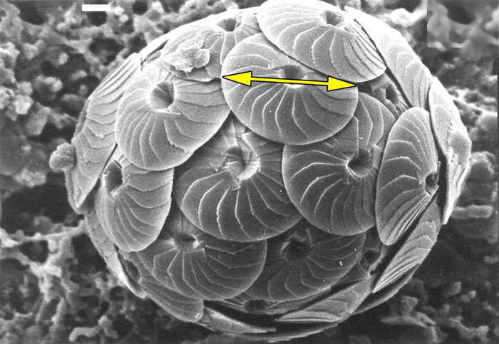
Figure 2. Stacked vertical slices through the density distribution model for C. leptoporus-C. macintyrei of Knappertsbusch (2000). The left panel shows color-coded stacks of near-baseline contours (2 specimens per grid-cell) of the model in "front view" (i.e., parallel to PCA I in figure 8 of Knappertsbusch, 2000). Slices are about 2 elements apart from each other. The uppermost slice (yellow to white) corresponds to the termination of the divergeing branch leading to morphotype D. The right panel shows color-coded stacks of near-baseline contours (2 specimens per grid-cell) in "side-view" (i.e., parallel to PCA II), at 1.02 units apart from each other (the slices correspond to those shown in figure 9 of Knappertsbusch, 2000). More than a decade ago this representation was the first view of the semi-continuous, four-dimensional hyperspace of the morphological variability in the C. leptoporus-C. macintyrei plexus. Though complicated, it gives an impression of the prominent divergence of extra-large coccoliths (morphotype D) between 12 Ma and 8 Ma.
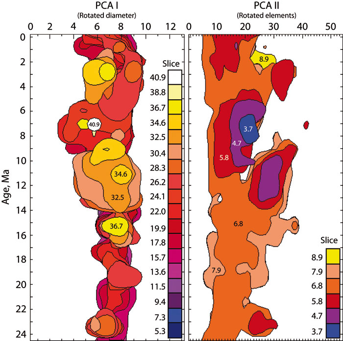
Figure 3. Globorotalia menardii in umbilical view. The calcitic shells of this planktonic foraminifer show considerable variation of the shell. Same specimen as illustrated in Knappertsbusch et al. (2009).
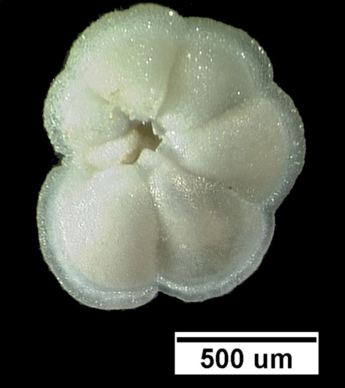
Figure 4. When seen in side view, globorotalid shells can be easily characterized by bivariate measurements of the spiral height (delta x) versus the length of the shell in keel view (delta y).
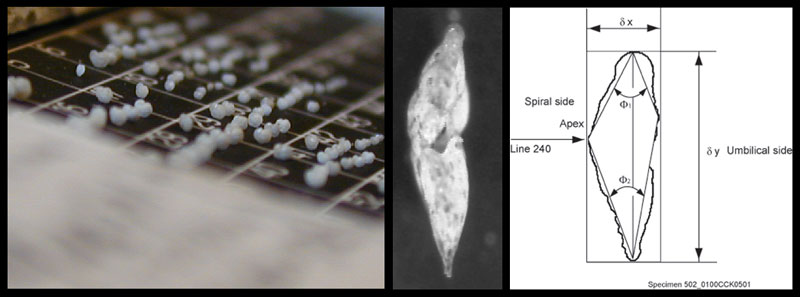
Figure 5. Flow-scheme of programs for the preparation of original data to a data model, that can be imported to Voxler for displaying frequency isosurfaces. See PDF version for zoomable version. Program names are written in bold and italics, input and output data are indicated in plane text.
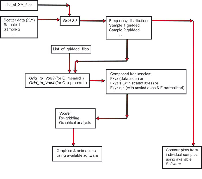
Figure 6. Steps from contoured bivariate data to interpolated iso-surfaces in the case of C. leptoporus. 1: Scatter plot of diameter versus elements from sample DSDP 251A-12-1, 88 cm. Grid-cells subdivide the diameter axis into intervals of 1 micrometer length and the diameter axis into intervals of 2 elements width. 2: Contoured absolute frequencies (see frequencies tabulated in Table 1 derived from scattered data shown in Figure 6.1 using the above grid-cell size of 1 micrometer x 2 elements). Contour intervals are 3 specimens per grid-cell. 3: Normalization of the axes. The center of each diameter interval is divided by 13.5 while the center of each element interval is divided by 53 (see text for further explanation). 4: A stack of contoured relative frequency distributions in the space of normalized diameter versus elements from three different geological times. The time axis is normalized by division of the age of each sample by the age of the oldest sample of the entire data set (i.e., 23.08 Ma). Between Figure 6.4 and Figure 6.5 absolute frequencies per sample were transformed into relative frequencies per sample. 5: Iso-surface after connecting outer contour lines of equal (relative) frequency throughout the complete set of C. leptoporus data. The illustrated iso-surface shows the evolution of rare coccoliths in the bivariate space of diameter versus number of elements. Increased frequencies of coccoliths are located inside the iso-surface. 6: Animated clips of the relative frequency iso-surface of C. leptoporus captured at changing stratigraphic levels (iso-surface values set to 1.52). Changing numbers in the lower right corner indicate the geological age in million years ago. To open an interactive animation please click here. Click here for viewing a flat, printable image series of the above animated scenes. The phylogenetic tree and positions of C. leptoporus-C. macintyrei morphotypes A, B, C, D, E, E', I, L and S (red letters) were taken from Knappertsbusch (2000) and projected into the animated iso-surface. Based on genetic evidence the extant morphotypes I and L are considered now as separate species Calcidiscus leptoporus and Calcidiscus quadriperforatus, respectively (Quinn et al., 2004), while the specific status of extant morphotype S is pending on documentation of its holococcolith bearing life-cycle phase (Quinn et al., 2003; Young et al., 2003).
PE NOTE: For opening this and the animations in the other figures, QuickTime Player should be installed for best performance.
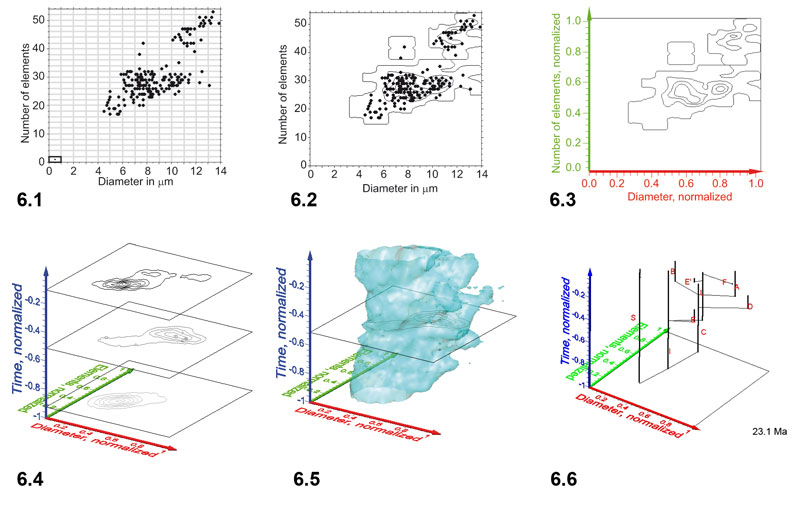
Figure 7. Steps from contoured bivariate data to interpolated iso-surfaces for G. menardii. 1: Scatter plot of spiral height versus axial width measurements (161 specimens) from sample DSDP 502A-1H-1, 15-20cm, which corresponds to the first sample in Figure 7 of Knappertsbusch (2007). 2: Contoured frequency plot of the data shown in Figure 7.1. delta X = 50 micrometers in X-direction and delta Y = 100 micrometers in Y-direction (see highlighted grid-cell in the lower left corner of Figure 7.1. Contour intervals are 2 specimens per grid-cell. Frequencies for this example are tabulated in Table 2. 3: Normalization of axes to unit values between 0 and 1. For this transformation the x-component (i.e., in direction of spiral height) of frequencies within each grid-cell was divided by 675 and by 1550 along the y-component (i.e., in direction of axial length). 4: A stack of contoured frequency diagrams from three different geological times. Notice that the time axis has been normalized to values between 0 and -1 by division of the age of each sample by the oldest sample age (8 Ma) of the data set described in Knappertsbusch (2007). Also, the absolute frequencies shown in Figure 7.2-3 were transformed into relative frequencies in Figure 7.4 for inter-sample comparison. 5: Iso-surface after connecting outer contour lines of equal relative frequency (isovalue of 1.28) throughout the complete set of G. menardii at DSDP Site 502A (Caribbean Sea). Frequent specimens are distributed inside the illustrated illustrated iso-surface, rare specimens are distributed towards the outer skin of the data body. 6: Animated clips of the relative frequency iso-surface of G. menardii at changing stratigraphic levels (iso-surface values set to 1.28) of DSDP Site 502A. Click here to open an interactive animation in a new window. Changing numbers in the lower right corner indicate the geological age in million years ago. 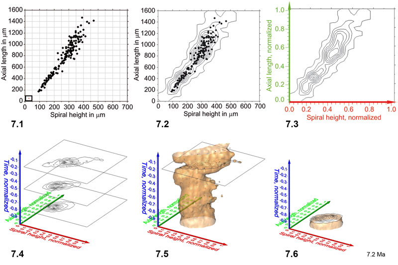
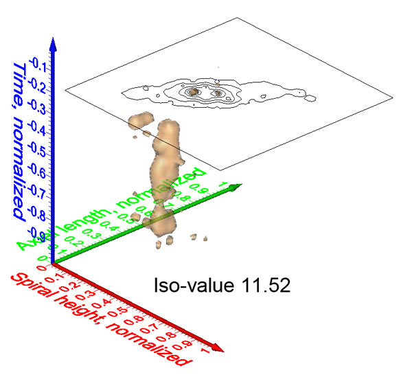
Figure 8. Spinning video animations of normalized density diagrams for a constant iso-value of 1.52 for C. leptoporus. All axes are normalized and represent diameter (red), number of elements (green) and time (blue). Click here 8.1, 8.2, and 8.3 to open and launch animations. 1 shows a solid iso-surface representation. Please notice the prominent and time-transgressive restriction of the density-surface (at about the level of the horizontal plane), which divides the model into a lower and an upper "valve." Click here for viewing a flat, printable image series of the animated scene of Figure 8.1. 2 shows the same iso-surface as in Figure 8.1 but in wireframe representation for a better visibility of the inserted phylogenetic tree. Click here for viewing a flat, printable image series of Figure 8.2. 3 illustrates the same data as shown in Figure 8.1, but as a wireframe diagram and spinning about a horizontal axis in order to show the iso-surface structure. Click here for viewing a flat, printable image series of Figure 8.3.
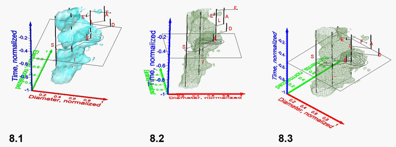
Figure 9.1-9.2 Spinning video animations of normalized density surface for G. menardii at Caribbean DSDP Site 502 (click here to launch animations 9.1 and 9.2. All axes are normalized and represent spiral height (red), axial length (green) and time (blue). Figure 9.1 shows a rotation cycle in counter-clockwise direction about a vertical spin-axis. A constant isovalue of 1.28 was selected to illustrate a low-frequency envelope of morphological trends through time in the spiral height versus axial length morphospace. Click here for viewing a flat, printable image series of Figure 9.1. Figure 9.2 shows the same iso-surface as in Figure 9.1 but rotating about a horizontal axis in direction towards the observer (click here for a printable, flat image series of the animated scene of Figure 9.2).
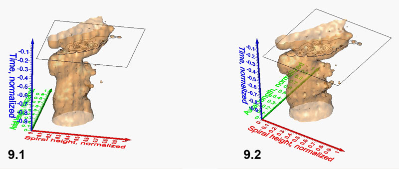
Figure 10.1-10.3. Iso-surfaces (isovalue=1.28) for G. menardii at the Caribbean DSDP Site 502 (Figure 10.1, which is the same model as shown in Figure 9) and DSDP Site 503 (Eastern Equatorial Pacific, Figure 10.2). Figure 10.3 shows involved iso-surfaces for both sites. Click here to launch animation of 10.3.
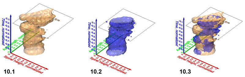
Figure 11.1-11.4. Frequency iso-surfaces for C. leptoporus coccoliths captured at increasing isovalues of 0.50 (Figure 11.1), 1.52 (Figure 11.2; same value as in Figure 8), 2.50 (Figure 11.3) and 4.00 (Figure 11.4). Axes are the same as in Figure 8.
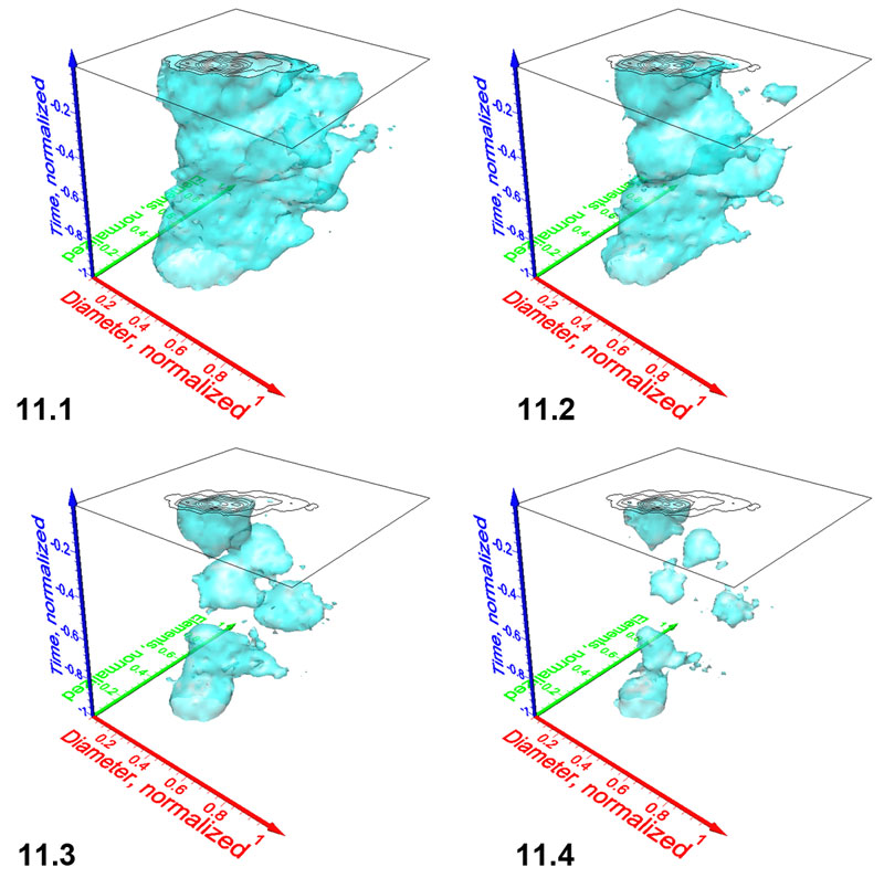
Figure 12.1-12.2. Pulsating diagrams of C. leptoporus in side view showing maximum coccolith variability (Figure 12.1) and in front view (Figure 12.2), where coccolith variability appears minimal. Axes are the same as in Figure 8. Click here to launch 12.1 and 12.2 animations. The projected phylogenetic dendrogram is the same as illustrated and discussed in Knappertsbusch (2000) and Knappertsbusch (2001). Numbers in the lower right corner of each animation indicate iso-value steps of 0.5.
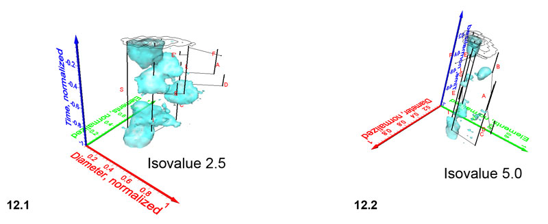
Figure 13.1-12.4. Iso-surfaces for frequencies of G. menardii at DSDP Site 502 taken at isovalues (normalized specimen densities) of 1.28, 4.90, 7.00 and 9.15, respectively. Axis names are the same as in Figure 9. The iso-surface for the value of 1.28 is also shown in the spinning diagrams in Figure 9.1 and 9.2.
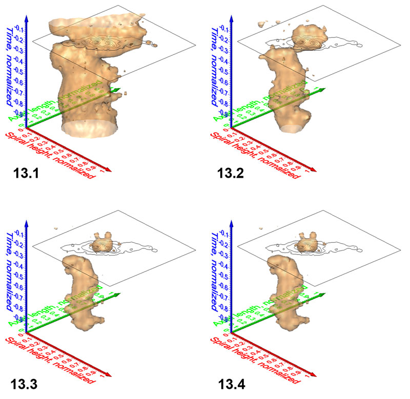
Figure 14. Animated sequence of frequency iso-surfaces for G. menardii at DSDP Site 502. Axis names are the same as in Figure 9. Click here to launch animation in a new window. Numbers in the lower right corner of the animation indicate iso-values at intervals of 1.28.
Michael W. Knappertsbusch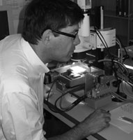 Natural History Museum Basel
Geology Department
Augustinergasse 2, 4001-Basel
Switzerland
Michael Knappertsbusch is curator for micropaleontology at the Natural History Museum in Basel. He studied geology at the Federal Institute of Technology (ETH) in Zürich, Switzerland, and graduated in 1986 with a micropaleontological diploma thesis about planktonic foraminiferal biostratigraphy in Northern Italy. In 1990 he obtained a PhD in Geology from ETH about coccolithophorids with a special emphasis on the morphological evolution of Calcidiscus leptoporus and related ancient forms. Residing in Amsterdam (Free University) from 1990 to 1994 he collaborated as a post-doc in the "Global Emiliania Modelling Initiative," a major investigation about the role of Emiliania huxleyi for the global carbon cycle.
Since 1994 he has been employed as curator for micropaleontology at the Natural History Museum in Basel (NMB), Switzerland. He runs the West-European Micropaleontological Reference Center of the DSDP and ODP and is responsible for all micropaleontological collections held at the NMB. His main research interest centers about patterns and biogeography of morphological evolution of oceanic microfossils, now mainly planktic foraminifera. Research includes the development of tools for morphometric investigations and visualization techniques for microfossils on the computer. An important recent breakthrough is the construction of an imaging system for automated foraminiferal orientation and imaging (AMOR) and software tools for automated shell measurements. These tools are employed by Michael and his current PhD student Yannick Mary for extended morphometric investigations of the Neogene planktic foraminifer Globorotalia menardii and related forms from a variety of deep-sea cores located in the Caribbean Sea, Eastern Equatorial Atlantic, off NW Brazil and from selected time-slices worldwide including the Holocene and Late Pliocene.
![]()
Yannick Mary Natural History Museum Basel
Geology Department
Augustinergasse 2, 4001-Basel
Switzerland
Yannick Mary began studying micropaleontology during his bachelor degree of geological oceanography at the University of Bordeaux, France. He completed his education there with a master's degree in paleoceanography, with a specialisation in climatic and environmental reconstructions with the help of planktonic foraminifera. In 2008 he graduated with a diploma thesis entitled "Populations of planktonic foraminifera in the Bay of Biscay: comparison of actual faunas with a fossil record covering the last 2000 years."
Thereafter, he felt the time has come for him to leave France and to go abroad. Since 2009, he has been working on his PhD at the Natural History Museum of Basel, Switzerland, under the supervision of Michael Knappertsbusch. His research is about mapping of the morphological variability of Pliocene menardiform globorotalids in order to better understand species-level diversity and speciation mechanisms in the marine plankton. For this purpose, he is working with an automatic device, the prototype robot AMOR, and he is heavily engaged with automation, informatics and programming next to his micropaleontological topic.
The research interests of Yannick Mary emerged from all the different aspects of his earlier education: Studying the morphological diversity of planktonic foraminifera and environment variability raised his special curiosity and interests in understanding the relationships between climate, environment and evolution of this special group of organisms.
Mining morphological evolution in microfossils using volume density diagrams
Plain Language Abstract
Morphometry is an important technique for the quantitative description of variations and differences between closely related extant and extinct species and their phylogenetic relationships. Morphotypes include a group of specimens that most typically describe the morphological appearance in a fossil assemblage. They are characterized by a combination of meaningful, independent morphological characters. In the ideal case morphotypes are recognizable as well separated data clusters in a multivariate set of morphometric measurements. In reality, however, there often exists overlap between such clusters and then statistical and/or graphical methods must be applied to best separate these clusters in a reliable way. Whether a morphotype also represents a biological species must further be clarified using independent evidence from biological, (paleo-) ecological, biogeographic, geochemical or molecular investigations. If the history of morphotype variation is studied in a sequence of successive samples in the geological record, moments of evolutionary splitting and divergence may be uncovered, which eventually witness speciation of an ancestral species into a descendent one. Such analysis, however, requires a very large number of measurements through time, from several locations. Understandably, these data are often difficult to analyze and interpret, even with the help of sophisticated statistical methods. Graphical analysis of the results is thus irreplaceable to reveal the morpho-phylogenetic relationships from one morphotype to another. In the present contribution a graphical analysis and display software called Voxler from Golden Software is exploited, which allows the communication of complicated morphological evolutionary trends through geological time to researchers and to laymen. Two pre-existing and published data sets for the study of evolution in these organisms are used for the present exercise: The first example is the plexus of Calcidiscus leptoporus – Calcidiscus macintyrei, a group of Neogene marine calcareous planktonic algae including morphologically closely related extinct and extant morphotypes. These algae produce minute calcite platelets – coccoliths – that surround the cell and which after death accumulate to thick piles of calcareous deep sea oozes at the bottom of the oceans. The second example is Globorotalia menardii, a representative of Neogene planktonic foraminifera, and which belongs to marine calcareous shell secreting planktonic protists. Also these shells - after settlement to the bottom of the ocean - are major contributors to worldwide deep-sea sediments. In both cases, the original observations consisted of simple bivariate measurements of the hardparts along a number of deep-sea cores, i.e., coccolith size versus its number of sinusoidal ornamentations on the distal side for C. leptoporus, and the length versus width of shells in profile view in the case of G. menardii. The time-series of bivariate measurements were transformed into discrete time-series of bivariate frequency distributions, which themselves were interpolated to obtain continuous density diagrams of specimens throughout the bivariate morphospace and through geological time. These density variations could then be displayed in three dimensions and animated using Voxler. The advantage of this graphical representation is that morphotype evolution could be analyzed and visualized more comprehensively than with any of the previously applied methods (i.e., stacked series of scatter- or contoured frequency plots from one time level to the next, or stacks of transversal sections of specimen frequencies parallel to the time axis, which were all quite difficult to present to the general audience). Using the animated density diagrams the authors are convinced, that they portray measured evolutionary patterns such as splitting and divergence more intuitively than without such tools.
Resumen en Español
Exploración de la evolución morfológica en microfósiles mediante el uso de diagramas de volumen-densidad
Se describe una técnica para visualizar series de medidas morfométricas bivariantes de conchas de microfósiles a través del tiempo geológico con ayuda de diagramas tridimensionales animados de distribución de volúmenes y densidades. Se han analizado dos series de datos previamente publicadas, una correspondiente a cocolitofóridos neógenos del grupo de Calcidiscus leptoporus-Calcidiscus macintyrei y la otra a foraminíferos planctónicos del plexo de Globorotalia menardii. La técnica consiste en la conversión de series de datos de medidas morfométricas discretas en distribuciones continuas de densidades de frecuencias, que pueden ser analizadas con la ayuda de Voxler, una herramienta de minería de datos gráficos creada por Golden Software. Esta herramienta permite crear y animar estructuras complejas a partir de las medidas morfométricas de los microfósiles facilitando una visualización intuitiva y de conjunto de la estructura y dinámica de los patrones evolutivos complejos. En combinación con las extensas series de datos morfométricos sobre microfósiles oceánicos de las que se dispondrá en un futuro próximo, este método puede servir para potenciar el estudio de aspectos tales como la evolución morfológica y la especiación y llegar a unas concepciones más universales de las especies, tan necesarias en los estudios paleontológicos. Una conclusión importante de este trabajo es que la distribución de las frecuencias de tamaño a lo largo del tiempo muestra una mayor diferenciación en conjuntos morfotípicos en el caso de los cocolitos que en el de los foraminíferos planctónicos. Esta diferencia se explica por las diferencias en el desarrollo ontogenético entre el alga C. leptoporus y el foraminífero G. menardii, lo que puede tener implicaciones en la clasificación de morfotipos y los estudios sobre la evolución a través de la morfometría de cocolitofóridos y foraminíferos.
PALABRAS CLAVE: microfósiles; Calcidiscus leptoporus; Globorotalia menardii; evolución morfológica; minería de datos; gráficos de volumen-densidad
Traducción: Miguel Company
Résumé en Français
Exploration de l'évolution morphologique des microfossiles par les diagrames volume-densité
Une nouvelle technique de visualisation de données morphométriques de tests de microfossiles à travers les temps géologiques est ici développée et décrite, basée sur l'animation 3D de distributions de volumes et de densités. Deux séries de données différentes, issues de résultats préalablement publiés, sont illustrées à l'aide de cette méthode, la première concernant le groupe de coccolithophoridés du Néogène Calcidiscus leptoporus-Calcidiscus macintyrei, la seconde portant sur le plexus spécifique du foraminifère planctonique Globorotalia menardii.
Cette technique s'appuie sur la conversion de séries de données de mesures morphométriques discrètes en distribution continue de densités de fréquences. Elle permet d'utiliser directement des mesures morphologiques de microfossiles, effectuées sur plusieurs niveaux de carottes correspondant à différents intervalles de temps. L'utilisation de l'outil graphique de data mining Voxler, créé par Golden Software, permet ensuite de créer et d'animer des diagrammes surfaciques complexes représentant les structures et motifs évolutifs au sein de ces distributions. Il est ainsi possible d'obtenir une visualisation des dynamiques évolutives complexes, immersive, intuitive et détaillée.
En combinaison avec l'arrivée future de données supplémentaires, issues de l'étude exhaustive des microfossiles océaniques actuels et fossiles, cette méthode possède un grand potentiel dans l'étude de domaines tel l'évolution morphologique et la spéciation, et pourrait contribuer à définir des concepts spécifiques plus précis et plus généralistes, dont la micropaléontologie a grand besoin.
De plus, une conclusion importante de cette expérience réside dans le fait que la distribution des fréquences à travers le temps est fondamentalement différente entre les espèces de coccolithes et de foraminifères planctoniques considérées. Il existe en effet une tendance à la différenciation morphologique en sous-ensembles morphotypiques plus importante chez C. leptoporus que chez G. menardii. Ce phénomène peut en partie être expliqué par des différences majeures au niveau ontogénique entre les deux groupes, ce qui peut avoir diverses implications en ce qui concerne la classification de morphotypes et les recherches sur l'évolution des coccolithophoridés et des foraminifères.
Mots-clefs: microfossiles, Calcidiscus leptoporus; Globorotalia menardii, évolution morphologique, exploration de données, diagrames volume-densité
Translator: authors and Loïc Costeur
Deutsche Zusammenfassung
Eine spezielle Technik zur verbesserten, räumlichen Darstellung morphometrischer Messungen von Mikrofossilien-Schalen mit Hilfe von 3D-animierten Volumen-Dichte Diagrammen wird vorgestellt.
Die Methode eignet sich hervorragend für die Untersuchung von komplexen Mustern der morphologischen Evolution, besonders im Falle von Mikrofossilien. Um das Potenzial von Volumen-Dichte Diagrammen aufzuzeigen werden zwei bereits existierende und publizierte morphometrische Mikrofossil-Datensets verwendet, im ersten Falle die Coccolithophoridengruppe Calcidiscus leptoporus-Calcidiscus macintyrei, im zweiten Falle die Neogene Foraminiferengruppe um Globorotalia menardii, welche ebenfalls ausgestorbene Formen beinhaltet. Die aufgezeigte Technik konvertiert bivariate Messungen von Schalen aus einer Probenserie in eine kontinuierliche bivariate Häufigkeitsverteilung durch die geologische Zeit hindurch, welche mit Hilfe der kommerziell erhältlichen Software Voxler von Golden Software räumlich in allen Schnittlagen dargestellt und animiert werden kann. Selbst im Falle der verhältnismässig einfachen bivariaten Natur der ursprünglichen Messungen können ausserordentlich komplexe Dichteverteilungen der Schalenhäufigkeiten im Raum der Messgrössen und durch die Zeit hindurch entstehen, so wie im Falle von C. leptoporus. Diese Muster sind mit den Methoden der multivariaten Statistik alleine nur sehr schwer interpretierbar, werden mit Hilfe der aufgezeigten Methode aber sofort verständlich. Die animierten Diagramme zeigen, wo sich möglicherweise morphologische Artbildung (durch Kladogenese) abgespielt hat, eine wichtigen Voraussetzung zur Erstellung von Artkonzepten und Phylogenien in der (Mikro-)Paläontologie. Interessanterweise hat sich bei den beiden Beispielen herausgestellt, dass im Falle der Coccolithophoriden C. leptoporus die Morphotypen viel stärker als separierbare Cluster differenzierbar sind als im Falle der planktonischen Foraminiferen G. menardii, wo mögliche Morphotypen stärker ineinander übergehen. Dieser Beobachtung wird durch die kontinuierliche Veränderung der Schalenmorphologie im Verlaufe der Ontogenie bei Foraminiferen erklärt, welche bei der Coccosphärenabdeckung in dieser Art und Weise nicht vorkommt. Diesem Unterschied zwischen dem Kalknannoplankton und den planktonischen Foraminiferen muss bei der morphometrischen Untersuchung der Evolution Rechnung getragen werden.
Translators: Authors
Arabic
Translator: Ashraf M.T. Elewa
-
-
-
Review: The Princeton Field Guide to Mesozoic Sea Reptiles
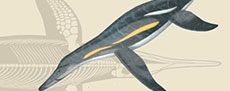 The Princeton Field Guide to Mesozoic Sea Reptiles
Article number: 26.1.1R
April 2023
 Poster Winners 2024