

Article Search
Volume 27.1
January–April 2024
Full table of contents
ISSN: 1094-8074, web version;
1935-3952, print version
Recent Research Articles
See all articles in 27.1 January-April 2024
See all articles in 26.3 September-December 2023
See all articles in 26.2 May-August 2023
See all articles in 26.1 January-April 2023
FIGURE 1. The experimental setup. 1.1 Picture of the water tank containing the burrowing environment. 1.2 Scheme of the setup. Shell models were placed at an initial position touching the sediment surface and then pulled in by two linear motors mounted vertically at the outside of the tank. The force was transmitted to the shell by two steel cables deviated by pulleys. By alternately pulling, the linear motors induced the typical rocking motion employed by burrowing bivalves. 1.3 Central metal disc and two 3D printed valves, outer and inner side. The valves were fixed to the metal disc by a bayonet coupling mechanism. The cables were attached to the shell at the two attachment arms of the metal disc. 1.4 Assembled shell. Pictures 1.1, 1.3 and 1.4 reprinted from Germann and Carbajal (2013). © IOP Publishing. Reproduced by permission of IOP Publishing. All rights reserved.
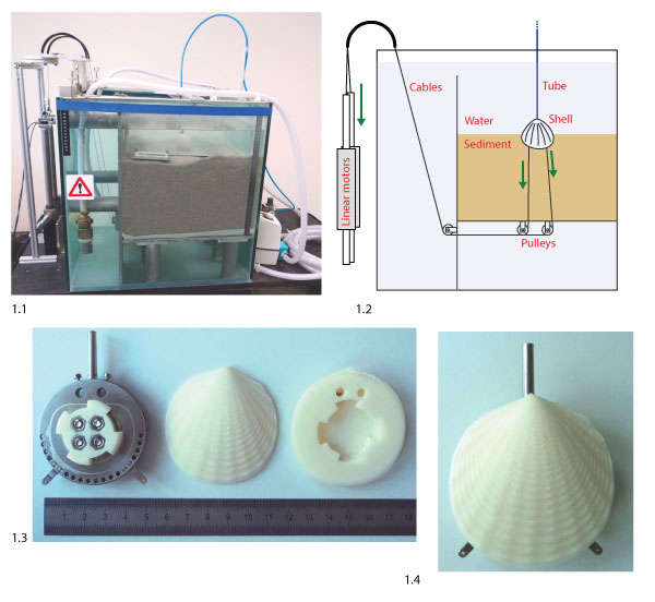
FIGURE 2. Geometrical model to generate artificial shell morphologies. 2.1 Illustration of the generation of a shell mesh, with n = 10 segments (black, dashed) and m = 10 growth steps (red, solid). The aperture curve was repeatedly scaled and rotated around axis d to generate the shell surface. 2.2 The sculpture profiles δr and δc used to generate radial (top) and commarginal ridges (bottom, ventral to the right). 2.3 Aperture curve of a shell (individual 6 in Figure 8), generated from parameters 1-8 in Table 1. The parameters define the polar coordinates of five points c1-c5 in the plane that span a control polygon (black) and define a NURBS curve (red). The aperture curve consists of a discretization of this curve into n points as in 2.1. The red arc denotes the position of the umbo and point A the position of the incircle of the aperture curve, where the attachment structure was placed (see text).
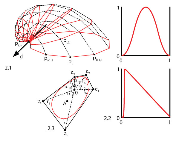
FIGURE 3. Example shell morphologies: 3.1 neutral, with a round aperture curve, intermediate values for all parameters and no sculpture (a = 0), 3.2 long aperture curve, 3.3 high aperture curve, 3.4 flat, with λ = 1.02069, 3.5 inflated, with λ = 1.00339, 3.6 featuring an ear, using an aperture curve with a large indentation, 3.7 with maximal commarginal frequency, 3.8 with medium commarginal frequency, 3.9 with minimal commarginal frequency, 3.10 with maximal radial frequency, 3.11 with medium radial frequency, 3.12 with minimal radial frequency, 3.13 with a radial-commarginal mixture, 3.14 featuring a sharp arrow shape, 3.15 with an arbitrary shape. Note that the scale is not the same for all shells.
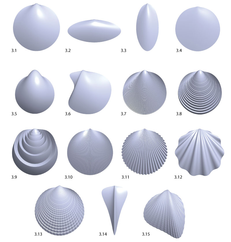
FIGURE 4. Different shell dimensions. While the width W is always defined as the dimension orthogonal to the aperture plane, the other two dimensions may be defined in different ways, cf. Table 2. The burrowing direction is downwards. 4.1 Length L and height H. Length is parallel to the hinge axis. 4.2 Tallness T and broadness B. Tallness is parallel to the burrowing direction, i.e., vertical. 4.3 Major axis length J and minor axis length N. J is along the largest diameter of the shell.
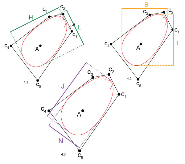
FIGURE 5. Burrowing depth boxplot. 20 generations of shells were generated. In each generation, the three new shells were evaluated and the two parents of the previous generation were re-evaluated (red labels). Each evaluation of a shell consisted of 10 repeated burrowing runs of which the final burrowing depths were measured. One box in the plot summarizes these 10 repetitions. The labels of the x-axis give the generation number (1-20) and the shell number (1-60).
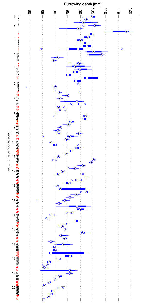
FIGURE 6. Depth correction. 6.1 Original depth data (blue, corresponds to the sequence of medians shown in Figure 5). The repeated evaluations are marked by red circles and connected by dashed lines. 6.2 Shift 1: depth data shifted such that repetitions match under the assumption that compaction is irreversible. 6.3 Shift 2: depth data shifted such that repetitions match and the final depth curve has a horizontal regression line. 6.4 The shift vectors shift 1 and shift 2 added to the original data to generate the corrected versions in 6.2 and 6.3.
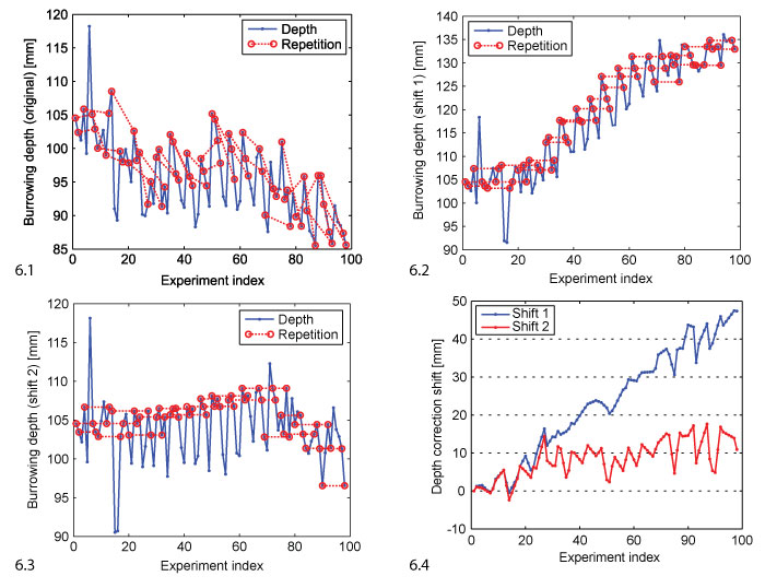
FIGURE 7. Fitness and mutation rate. 7.1 The plot shows the range of fitness values for each generation. The solid line follows the best individual of each generation. The dark shaded area covers the best two individuals, i.e., the selected ones, the bright shaded area covers all individuals. The original data is compared to two versions corrected in analogy to the depth values in Figure 6. 7.2 The same kind of range evolution plot for the mutation rate.
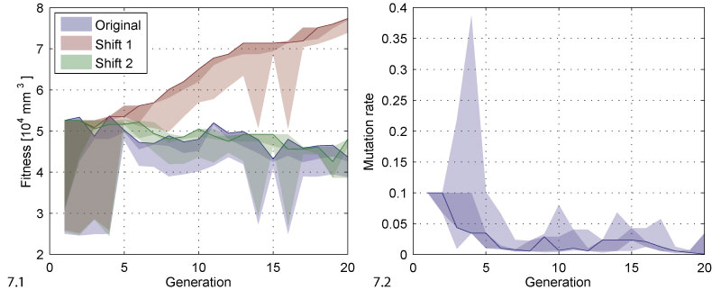
FIGURE 8. Phylogenetic tree. Each row corresponds to a generation. A generation contains three new individuals generated by reproduction and two re-evaluated individuals selected in the last generation. As reproduction operators, mutation (red dotted lines) and crossover + mutation (blue dashed lines) were used.
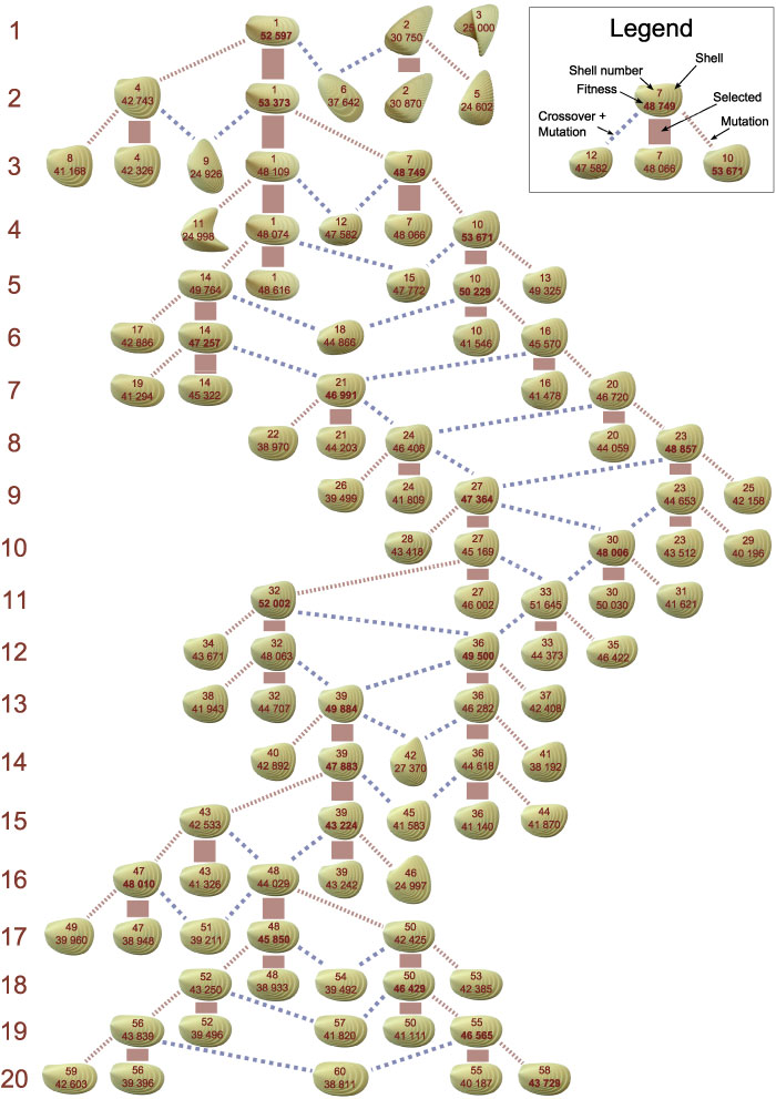
FIGURE 9. Parameter range evolution. The plots show how the parameters changed during evolution. The solid line follows the best individual, the dark shaded area covers the selected individuals, the bright shaded area covers all individuals. The red dots represent shells that were generated but discarded because they were invalid, i.e., because they did not result in printable shell morphologies. The range of the y-axis corresponds to the range of the respective parameter.
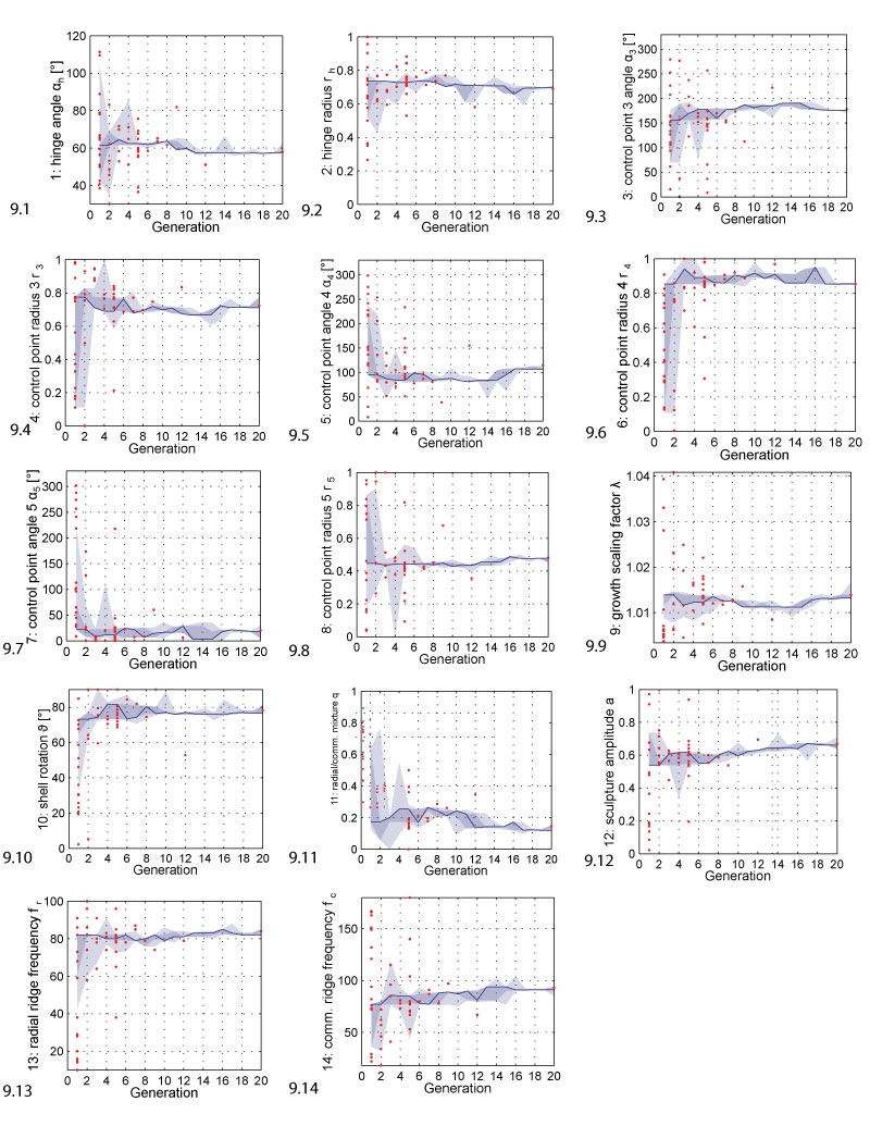
FIGURE 10. Phenotypic parameter range evolution. The plots show how the phenotypic parameters changed during evolution. The solid line follows the best individual, the dark shaded area covers the selected individuals, the bright shaded area covers all individuals.
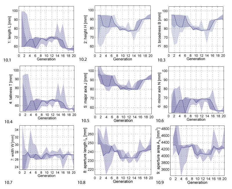

TABLE 1. Genetic parameters from which the shell morphology was generated. Parameters 1-10 defined the overall shape of the shell, parameters 11-14 the surface sculpture. The shape of the aperture curve used 8 parameters, see Figure 2.3. For the effect of parameters λ, q, fr and fc, see Figure 3. By reducing parameter a from 1 to 0, the sculptures of the sculptured examples in Figure 3 would be linearly reduced to a smooth surface.
|
Variable |
Range |
Parameter description |
|
|
1 |
αh |
[30°, 120°] |
hinge angle |
|
2 |
rh |
[0, 1] |
hinge radius |
|
3 |
α3 |
[0°, 360° –αh] |
angle of 3rd control point |
|
4 |
r3 |
[0, 1] |
radius of 3rd control point |
|
5 |
α4 |
[0°, 360° –αh] |
angle of 4th control point |
|
6 |
r4 |
[0, 1] |
radius of 4th control point |
|
7 |
α5 |
[0°, 360° –αh] |
angle of 5th control point |
|
8 |
r5 |
[0, 1] |
radius of 5th control point |
|
9 |
λ |
[1.00339, 1.04086] |
growth scaling factor |
|
10 |
ϑ |
[0°, 90°] |
shell rotation towards anterior |
|
11 |
q |
[0, 1] |
radial/commarginal mixture |
|
12 |
a |
[0, 1] |
sculpture amplitude |
|
13 |
fr |
[10..100] |
radial ridge frequency |
|
14 |
fc |
[18..180] |
commarginal ridge frequency |
TABLE 2. Phenotypic (morphometric) parameters. In addition to the parameters listed in Table 1 that were used to generate the shells, we used this set of phenotypic parameters computed from the final shells to find possible correlations with the fitness.
|
Variable |
Unit/Range |
Parameter description |
|
|
1 |
L |
[mm] |
length, dimension parallel to hinge axis |
|
2 |
H |
[mm] |
height, dimension orthogonal to length |
|
3 |
B |
[mm] |
broadness, dimension orthogonal to burrowing direction |
|
4 |
T |
[mm] |
tallness, dim. parallel to burrowing direction |
|
5 |
J |
[mm] |
major axis length, largest diameter |
|
6 |
N |
[mm] |
minor axis length, dimension orthogonal to major axis |
|
7 |
W |
[mm] |
width, dimension orthogonal to aperture plane (over both valves) |
|
8 |
lA |
[mm] |
aperture curve length, circumference of aperture |
|
9 |
AA |
[mm2] |
aperture area |
|
10 |
γ |
[0, 1] |
non-convexity, part of aperture area bending inwards |
|
11 |
pu |
[0, 1] |
relative umbo position (along L) |
|
12 |
pc |
[0, 1] |
relative centre position (along L) |
|
13 |
S1 |
[0, 1] |
streamlining, (Watters, 1993, based on L and H) |
|
14 |
S2 |
[0, 1] |
streamlining, (Watters, 1993, based on B and T) |
|
15 |
S3 |
[0, 1] |
streamlining, average angle between faces and burrowing direction |
TABLE 3. Correlations of genetic and phenotypic parameters and the burrowing depth D with fitness (original and shift 2, see Figure 6). We computed Pearson and Spearman correlation. The p-values and the correlation coefficients r are given.
|
Pearson correlation |
Spearman correlation |
|||||||
|
Fitness (orig.) |
Fitness (shift 2) |
Fitness (orig.) |
Fitness (shift 2) |
|||||
|
Variable |
p-value |
r |
p-value |
r |
p-value |
r |
p-value |
r |
|
D – T |
3E-40 |
0.92 |
4E-29 |
0.85 |
0 |
0.84 |
6E-08 |
0.52 |
|
T |
2E-14 |
-0.68 |
0 |
-0.73 |
5E-03 |
-0.28 |
5E-03 |
-0.28 |
|
L |
3E-10 |
-0.58 |
7E-12 |
-0.62 |
0.14 |
-0.15 |
0.18 |
-0.14 |
|
S2 |
6E-10 |
-0.57 |
2E-11 |
-0.62 |
9E-03 |
-0.26 |
9E-03 |
-0.26 |
|
lA |
4E-08 |
-0.52 |
2E-09 |
-0.56 |
2E-04 |
-0.37 |
1E-04 |
-0.38 |
|
pc |
5E-08 |
0.52 |
8E-10 |
0.57 |
0.3 |
0.11 |
0.3 |
0.1 |
|
fr |
6E-08 |
0.51 |
6E-09 |
0.55 |
0.55 |
0.06 |
0.93 |
0.01 |
|
S1 |
9E-07 |
-0.47 |
1E-07 |
-0.5 |
0.19 |
-0.13 |
0.21 |
-0.13 |
|
α5 |
1E-06 |
-0.47 |
2E-08 |
-0.53 |
0.06 |
-0.19 |
0.03 |
-0.22 |
|
α4 |
2E-06 |
-0.46 |
2E-08 |
-0.53 |
0.01 |
-0.26 |
2E-03 |
-0.31 |
|
S3 |
5E-06 |
0.44 |
2E-06 |
0.46 |
0.25 |
0.12 |
0.15 |
0.15 |
|
r4 |
2E-05 |
0.42 |
7E-07 |
0.48 |
0.38 |
0.09 |
0.17 |
0.14 |
|
γ |
5E-05 |
-0.4 |
5E-06 |
-0.44 |
0.06 |
0.19 |
0.02 |
0.24 |
|
rh |
1E-04 |
0.37 |
2E-06 |
0.46 |
2E-03 |
0.31 |
4E-06 |
0.45 |
|
α3 |
4E-04 |
0.35 |
3E-05 |
0.41 |
0.44 |
-0.08 |
0.37 |
-0.09 |
|
J |
5E-04 |
-0.35 |
2E-04 |
-0.37 |
3E-03 |
-0.3 |
2E-03 |
-0.31 |
|
B |
1E-03 |
0.33 |
5E-04 |
0.35 |
0.48 |
0.07 |
0.49 |
0.07 |
|
H |
1E-03 |
0.33 |
5E-04 |
0.35 |
0.68 |
0.04 |
0.76 |
0.03 |
|
q |
4E-03 |
-0.29 |
8E-04 |
-0.33 |
0.07 |
0.18 |
3E-03 |
0.3 |
|
r3 |
6E-03 |
0.28 |
2E-03 |
0.31 |
0.86 |
0.02 |
0.72 |
-0.04 |
|
λ |
0.02 |
0.24 |
0.01 |
0.25 |
0.45 |
-0.08 |
0.23 |
-0.12 |
|
D |
0.03 |
0.23 |
0.01 |
0.26 |
7E-07 |
0.48 |
2E-04 |
0.37 |
|
a |
0.03 |
-0.22 |
0.02 |
-0.24 |
2E-04 |
-0.37 |
1E-06 |
-0.47 |
|
ϑ |
0.04 |
0.21 |
6E-03 |
0.28 |
0.46 |
-0.08 |
0.39 |
-0.09 |
|
AA |
0.04 |
-0.21 |
0.04 |
-0.21 |
0.03 |
-0.22 |
0.04 |
-0.2 |
|
N |
0.08 |
-0.18 |
0.05 |
-0.2 |
0.41 |
-0.08 |
0.41 |
-0.08 |
|
αh |
0.22 |
-0.13 |
0.3 |
-0.11 |
0.28 |
0.11 |
0.04 |
0.21 |
|
r5 |
0.24 |
-0.12 |
0.26 |
-0.11 |
0.02 |
-0.23 |
0.03 |
-0.22 |
|
pu |
0.27 |
0.11 |
0.2 |
0.13 |
0.02 |
-0.24 |
3E-03 |
-0.3 |
|
fc |
0.38 |
0.09 |
0.18 |
0.14 |
0.2 |
-0.13 |
0.06 |
-0.19 |
|
W |
0.48 |
-0.07 |
0.42 |
-0.08 |
0.12 |
0.16 |
0.11 |
0.16 |
 Daniel P. Germann
Artificial Intelligence Laboratory
Department of Informatics
University of Zürich
Andreasstrasse 15
8050 Zürich
Switzerland
germann@ifi.uzh.ch
Daniel Germann received his Master's degree in computer science from the Swiss Federal Institute of Technology (ETH) in Zurich in 2007. His major was scientific computing, his minor artificial intelligence. Daniel Germann will shortly conclude his Ph.D. at the Artificial Intelligence Laboratory at the University of Zurich, which he started in 2008.

 Wolfgang Schatz
Academic Services Centre
University of Lucerne
Pfistergasse 2
6003 Luzern
Switzerland
Wolfgang.Schatz@unilu.ch
Wolfgang Schatz is a invertebrate paleontologist. He received degrees from the University of Zurich. For ten years he was senior researcher at the Paleontological Institute and Museum of the University of Zurich. His current research is on palecology and stratigraphy of fossil bivalves, especially on Middle Triassic flat clams.
 Peter Eggenberger Hotz
Mærsk-McKinney-Møller Institute
University of Southern Denmark
Campusvej 55
5230 Odense M
Denmark
petereggenbergerhotz@gmail.com
Peter Eggenberger Hotz received his medical degree in 1985 from the University of Zurich and his Ph.D. at the Artificial Intelligence Laboartory at the University of Zurch in 1999. He worked as a researcher on different projects in the fields of artificial evolution, self-assembly, artificial vesicles and genetic programmability. From 2006 to 2012, he was associate professor for Artificial Intelligence at the Mærsk-McKinny-Møller Institute, University of Southern Denmark.
Artificially evolved functional shell morphology of burrowing bivalves
Plain Language Abstract
The evolution of bivalve shell shapes is documented by a rich fossil record. In burrowing species, it is believed that the shell shape and surface structure play an important role for the burrowing performance. While the dimensions and features of shell shapes of different species have been measured thoroughly, there are almost no studies physically testing their actual effect in the burrowing process. To do this, we built an experimental setup. A printer that prints three dimensional (3D) objects was used to manufacture different shell models. We performed the first ever experiment to artificially evolve an optimal bivalve shell shape for burrowing. The result was a vertically flattened shell occupying only the top sediment layers. The major drawback of the setup was the difficulty to return the sediment into a similar state before each experiment. Nevertheless, it is demonstrated that palaeontological research may profit from an "understanding-by-building" approach. We suggest investigating bivalve shapes not only by simulating the burrowing process but also their evolution.
Resumen en Español
Evolución artificial de la morfología funcional de la concha de bivalvos excavadores
La evolución morfológica de los bivalvos está documentada por un abundante registro fósil. Se supone que la forma de la concha y la ornamentación juegan un papel importante en la actividad excavadora de las especies endobentónicas. Aunque se han llevado a cabo estudios morfométricos detallados de las conchas de los bivalvos, no existen apenas experimentos que evalúen sus propiedades dinámicas. Con objeto de analizar la morfología funcional de la concha de los bivalvos hemos empleado una metodología sintética y construido una configuración experimental para simular el proceso de excavación. Mediante el uso de un algoritmo evolutivo y una impresora tridimensional se ha llevado a cabo, por primera vez, una evolución artificial de la concha de un bivalvo. El resultado fue una concha aplastada verticalmente que ocupaba sólo las capas más superficiales del sedimento. El insuficiente control del sedimento ha sido la mayor limitación de la configuración y ha limitado el valor de los resultados. Sin embargo, se ha podido demostrar que la investigación paleontológica sistemática puede beneficiarse sustancialmente de los métodos sintéticos. Se conclute que la investigación de la morfología funcional no debe limitarse a reproducir los procesos dinámicos sino que debe tenerse en cuenta también la presión evolutiva mediante el uso de algoritmos evolutivos.
Palabras clave: bivalvos excavadores; morfología funcional; evolución artificial; presión evolutiva; biomecánica; morfoespacios
Traducción: Miguel Company
Résumé en Français
Morphologie fonctionnelle de coquille de bivalves fouisseurs artificiellement évolué
L'évolution morphologique des bivalves est documentée par un riche registre fossile. On pense que la forme de la coquille et de la sculpture de surface jouent un rôle important pour la performance d'enterrement des espèces endobenthiques. Alors que les études morphométriques détaillées de coquilles bivalves ont été faites, il n'y a presque pas d'études qui essaient expérimentalement leurs propriétés dynamiques. Pour étudier la morphologie fonctionnelle de la coquille des bivalves, nous avons utilisé une méthodologie de synthèse et construit un dispositif expérimental pour simuler le processus d'enterrement. En utilisant un algorithme évolutif et une imprimante 3D, la première évolution artificielle d'une coquille de bivalve a été effectuée. Le résultat a été une coquille aplatie verticalement occupant seulement les couches de sédiments du dessus. Le contrôle insuffisant des sédiments a été la principale limite de l'installation et a limité la portée des résultats. Néanmoins, il est démontré que la recherche paléontologique systématique peut sensiblement bénéficier de méthodes synthétiques. Nous suggérons de rechercher la morphologie fonctionnelle non seulement en imitant des processus dynamiques, mais aussi la pression évolutive en utilisant des algorithmes évolutionnaires.
Mots-clés: bivalves fouisseurs; morphologie fonctionnelle; évolution artificielle; pression évolutive; biomécanique; espaces morphologiques.
Translator: Kenny J. Travouillon
Deutsche Zusammenfassung
Mittels künstlicher Evolution erzeugte funktionelle Schalenmorphologie von grabenden Muscheln
Die morphologische Evolution von Bivalven ist durch eine grosse Menge von Fossilien dokumentiert. Es wird angenommen, dass Gehäusegestalt und Oberflächenskulptur eine wichtige Rolle beim Grabverhalten der endobenthischen Arten spielen. Während einige detaillierte morphologische Untersuchungen über Muschelschalen durchgeführt wurden, gibt es fast keine experimentellen Studien zu ihren dynamischen Eigenschaften. Um die Funktionsmorphologie der Muschelschale zu untersuchen setzten wir eine synthetische Methode ein und entwickelten einen Versuchsaufbau, um den Grabprozess zu simulieren. Anhand eines evolutionären Algorithmus und eines 3D-Druckers wurde die allererste künstliche Evolution einer physischen Muschelschale vorgenommen. Das Ergebnis war ein vertikal abgeflachtes Gehäuse, das nur die obersten Sedimentschichten okkupierte. Unzureichende Kontrolle des Sediments war die größte Limitierung des Aufbaus und beschränkte die Aussagekraft der Ergebnisse. Dennoch wurde gezeigt, dass Forschung über systematische Paläontologie erheblich von synthetischen Methoden profitieren kann. Wir empfehlen funktionelle Morphologie nicht nur durch Nachahmen dynamischer Prozesse zu untersuchen sondern auch durch Nachahmen von evolutionärem Druck indem evolutionäre Algorithmen genutzt werden.
Schlüsselwörter: grabende Bivalven; Funktionsmorphologie; künstliche Evolution; evolutionärer Druck; Biomechanik; Morphospaces
Translator: Eva Gebauer and author
Arabic
Translator: Ashraf M.T. Elewa
-
-
-
Review: The Princeton Field Guide to Mesozoic Sea Reptiles
 The Princeton Field Guide to Mesozoic Sea Reptiles
Article number: 26.1.1R
April 2023
 Poster Winners 2024