FIGURE 1. Orientation of measurement planes with respect to the tooth. The red area signifies the surface area scanned by OCT.

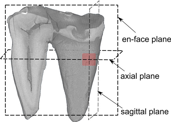
FIGURE 2. Specimen GS 26-1. Root of a right lower M1 of a senile individual of Ursus ingressus from Gamssulzen cave (Lower Austria). 2.1. Comparison between 3D volume rendering of µ-CT and OCT (λ _c =850 nm) data. 2.2. - 2.4. Axial cross sections of the mesial root by µ-CT at position i)-iii) as depicted in 2.1. The regions marked in red show the area scanned by OCT presented in Figure 3.

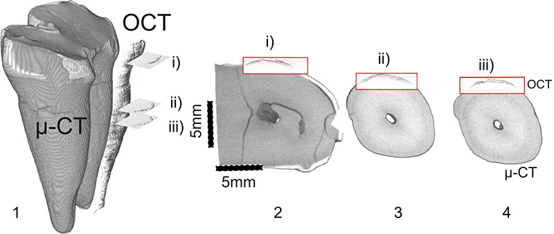
FIGURE 3. Specimen GS 26-1.Comparison between axial cross-sectional µ-CT and OCT (λ _c =850 nm) images on the distal root at position i-iii, as depicted in Figure 1. 3.1. The cross section close to the collum dentis shows enamel but no annuli. 3.2.-3.3. The cross-sectional images ii) and iii) show annuli.

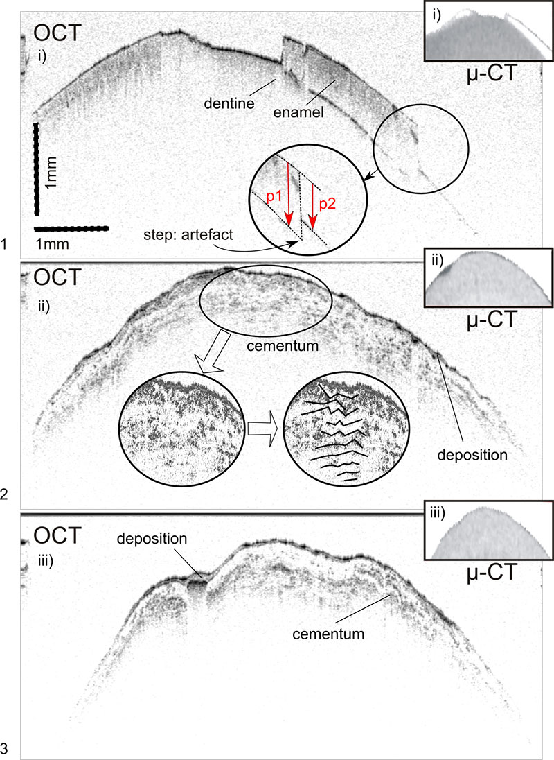
FIGURE 4. Specimen GS 26-1. 4.1. Volume rendering of the 3D µ-CT. The red area marks the region scanned by OCT. 4.2. Sectional view of 3D OCT data. (see animations for OCT scan). 4.3. µ-CT axial cross-sectional scans and 4.4. µ-CT en-face scan. (see animations for animated µ-CT scan).

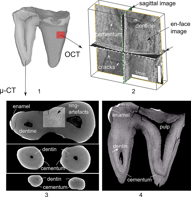
FIGURE 5. Axial cross-sectional OCT image (λ _c =1300 nm) in the lower third of the tooth radix of specimen. 5.1. GS 26-1 (distal). 5.2. GS 108-1 (mesial). 5.3. GS 108-2 (mesial). The camera images on the left show the OCT scanning region. The OCT images have a lateral dimension of 4 mm. The depth scale bar is stretched according to a refractive index of 1.6, leading to an image depth of about 1mm. The microscope images are 1x1 mm² in true aspect ratio. The depth scale of OCT images and microscope image is identical.

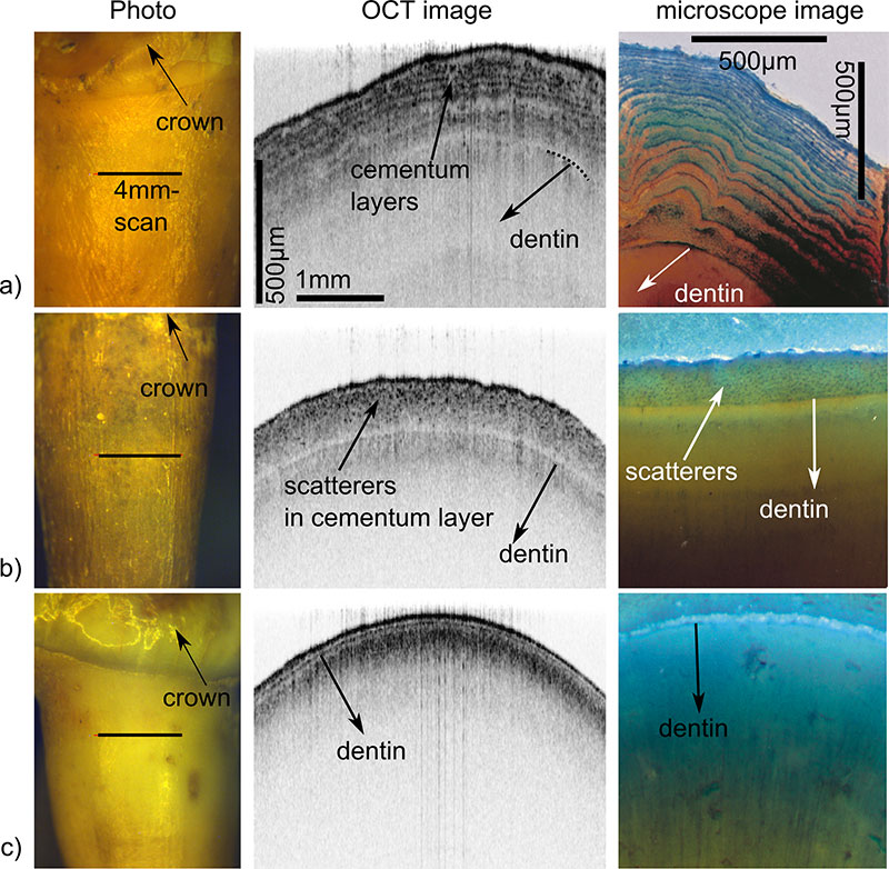
FIGURE 6. 6.1-2: Comparison between the commercial system at 1300 nm (6.1) and the Lab system at 800 nm (6.2), exemplified by cross-sectional images of the specimen GS 26-1. The arrow in 6.2 indicates a fine structure that cannot be resolved by the 1300 nm system. 6.3-4: Comparison between the commercial system (6.3) and the PS-OCT system at 1500 nm, exemplified by by cross-sectional images of the specimen GS 108-2. 6.4. shows the reflectivity image, and 6.5. the retardation image. The arrow in 6.3 indicates an annual ring, while the arrows in 6.5 indicate birefringence of the tooth.

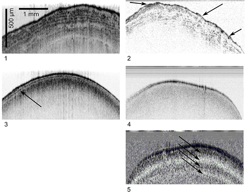
FIGURE 7. Specimen GS 108-2, right lower m1 of a young adult individual of Ursus ingressus from Gamssulzen cave (Lower Austria). Comparison between 7.1. transmitted pulse amplitude, 7.2. time delay of THz measurement and 7.3. µ-CT.

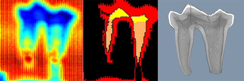
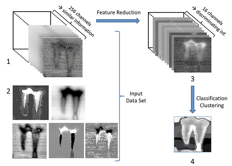
FIGURE 8. Image processing and hyper spectral data analysis: 8.1. Combined input data set containing hyper spectral data; 8.2. Overall features (main amplitude, phase slope, phase intercept, echo pulse delay, wavelet scaling factor); 8.3. Reduced feature set after applying the wavelet based feature reduction method; 8.4. Result of automatic classification by applying the two step partitional clustering method (k=20) based on the reduced feature set. For comparison: see animation of the result applying a Preclustering-based agglomerative hierarchical clustering method (40 clusters and 100 preclusters).