APPENDIX 1.

Use of the program HETEROSIM, and exercises for students.

The computer program HETEROSIM constructs geometrical shapes using the equations presented in this paper. The graphical construction is achieved by drawing opaque ellipses to represent successive positions of the whorl, with those nearest the viewer drawn last to create a rough impression of a solid 3D form. This graphical style is regarded as being satisfactory, but close inspection does reveal minor anomalies in the vicinity of the coiling axis. Other authors have produced renderings that are smoother and with a technically superior 3D appearance (e.g., Hammer and Bucher 2005; Noshita 2012), but this is thought to be unnecessary for current purposes, and in some respects the graphical style used here is clearer. HETEROSIM is restricted to simulations with elliptical whorl sections; this is thought to be appropriate, as attempting to find fits to other whorl shapes would be time-consuming and not relevant to the task of modelling heterochronic change in gross shell shape.

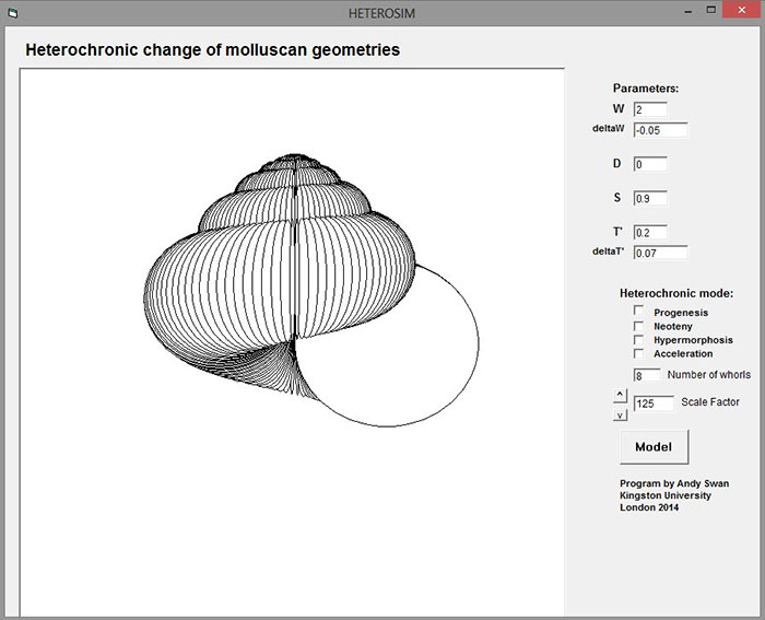
The user of the program is presented with eight boxes containing values that can be user-specified prior to heterochronic modelling: these are the six parameter values described in this paper, plus the number of whorls and a relative scale factor (see Appendix 2). The default values are those used in Figure 4. Clicking on the “MODEL” button then generates the simulation using the current parameters. (N.B. The parameters defined in this paper as W₀ and T’₀ appear on-screen as “W” and “T’”.)

The effect of heterochronic modes can then be simulated by clicking on the box(es) corresponding to the desired mode(s) (this will produce a “tick” in the box), and clicking on the “MODEL” button again. Repeated increments of the same or other modes can be executed. The modes can be de-selected by clicking on the ticked boxes. (For the sake of simplicity, and ease of use in a pedagogic environment, this version of the program offers only the default values for heterochronic change that are detailed in the main text of this paper.)

When the effect of heterochronic modes are modelled, the values of the parameters are updated. In one modelling experiment, it is expected that the user will not manually adjust the parameter values (except perhaps the scale factor) after setting-up the initial values.

The appropriate scale factor for the initial simulation is estimated by the program on the basis of the initial parameter values, but may nevertheless need to be adjusted. After applying heterochronic changes, the size of the simulated shell very often changes substantially. The scale factor can be adjusted readily by clicking on the “^” or “v” buttons. When this is done, all current heterochronic mode selections are switched off.

There is no special provision for capturing and printing graphics; the familiar <CTRL><ALT><PRNT SCRN> key combination can be used, or import facilities in graphics editing software.

The program should work on all PCs with Microsoft Windows or Windows emulation. It may be found that the program doesn’t initially run, and an error is shown that reports a missing Dynamic Link Library (.DLL) file. If so, this file can readily be found on the Microsoft web site and installed easily and free of charge. Users in European countries may need to change the decimal separator from a dot to a comma.

Exercises for Students

Initially, students should become familiar with the geometric parameters in the isometric case. Parameters Δ W and Δ T’ should both be set to zero, and W, T’, S and D adjusted (one at a time) so that the effect of each can be noted (this is good practice in gaining familiarity with any computer simulation). This can lead to more structured investigation:

1. Students should be introduced to the concept of morphospace, and a two-dimensional array of forms could be produced in the style of figure 2.2.3.1 in Swan (2001), perhaps with D and S kept constant and simulations with various permutations of W and T’ produced.

2. Students can then be given the task of finding parameter combinations that yield simulations similar to actual specimens. Illustrations of a range of specimens could be presented; these could include one or two allometric forms so that the key difference can be observed. Students should find that the adjustments required in order to more closely simulate isometric forms is quite intuitive. The failure to simulate allometric forms is instructive.

3. Students could be invited briefly to experiment with heterochronic changes on isometric forms. They will observe that there is no change in shape, even when there is change of size (in the case of progenesis and hypermorphosis).

Students can then be given the task of optimising all six parameter values for a given real allometric form. Members of the Pulmonata are good for this, especially the more typical members of the Helicidae. This optimisation is likely to be difficult, as this constitutes a search of six-dimensional morphospace, without an easy intuition of the direction in which the optimum lies. This is typical of the difficulty encountered when undertaking optimisation using models with large-dimensional parameter space in general.

4. Using a set of parameter values supplied by the instructor (perhaps the ones used in Figures 4, 5 and 6), students can experiment with the effect of the heterochronic modes. (In order to return to the starting point, they should note that an increment of neoteny can be reversed by an increment of acceleration and vice versa, and likewise for progenesis and hypermorphosis). They should attempt to understand how the “descendant” forms have resulted from the modification of the “ancestral” ontogeny.

5. For a more extended project, students could locate a source of illustrations of allometric gastropods from a specific taxonomic group (perhaps at Family level) and find the six optimal parameter values for one of the species (it is probably best to use one of the more conservative forms). A range of heterochronic “descendants” can then be produced for comparison with the variety of forms that actually occur. The plausibility of the heterochronic hypothesis for that group can then be critically assessed. (Note that, ideally, the phylogeny of the specimens in the chosen taxonomic group would be known, but this information is seldom available).

6. For more advanced study, students could be invited to consider the possible functional performance of the various forms and the ecology of the specified taxonomic group, and reach a verdict on whether heterochrony might be the means of producing a better-performing adult shape, or whether the “descendant” adult shape is merely a consequence of the favourability of evolutionary change in rates and timings in ontogenetic development.

APPENDIX 2.

“Screenshot” of the HETEROSIM program, as presented to the user.