

 Accounting for differences in element size and homogeneity when comparing Finite Element models: Armadillos as a case study
Article number: 19.2.2T
https://doi.org/10.26879/609
Copyright Palaeontological Association, August 2016
Author biographies
Plain-language and multi-lingual abstracts
PDF version
Submission: 27 October 2015. Acceptance: 4 July 2016
{flike id=1548}
ABSTRACT
Computing the average Von Mises stress of Finite Element Models to obtain a single measurement that represents the relative strength of vertebrate structures has been used recently in different works in palaeobiology. However, due to the nature of the Finite Element Analysis (FEA) data, which depends on the size of the elements of the mesh, this approach needs to be fully developed taking into account this influence of the size elements in the results. In this work, we proposed a Mesh-Weighted Arithmetic Mean as the adequate central tendency statistic for non-uniform meshes. On the other hand, when other statistical tools are used, we propose a Quasi-Ideal Mesh that takes into account the differences in size of the elements. Firstly, in order to analyse our proposed approach, one Cingulata mandible has been used generating different meshes. Afterwards, FEA has been applied in a case study in 20 different mandibles belonging to 14 species of Cingulata. Our results suggest that the proposed methodologies are suitable to compare different patterns of stress distribution. In particular, the methods proposed have been shown to be extremely useful when analysing the biomechanics of vertebrate bone structures that can be modelled as planar models in an interspecific comparative framework.
Jordi Marcé-Nogué. Universitat Politècnica de Catalunya - BarcelonaTech, 08222, Terrassa, Spain. jordi.marce.nogue@gmail.com
Soledad de Esteban-Trivigno. Transmitting Science, Gardenia 2, Piera, 08784, Spain; and Institut Català de Paleontologia Miquel Crusafont, Edifici ICP, Campus de la UAB s/n, 08193, Cerdanyola del Vallès, Spain. soledad.esteban@transmittingscience.org
Christian Escrig. Universitat Politècnica de Catalunya - BarcelonaTech, 08222, Terrassa, Spain. christian.escrig@upc.edu
Lluís Gil. Universitat Politècnica de Catalunya - BarcelonaTech, 08222, Terrassa, Spain. lluis.gil@upc.edu
Keywords: finite element analysis; mandible mechanics; biomechanics; diet; armadillos; functional analysis
Final citation: Marcé-Nogué, Jordi, de Esteban-Trivigno, Soledad, Escrig, Christian, and Gil, Lluís. 2016. Accounting for differences in element size and homogeneity when comparing Finite Element Models: Armadillos as a case study. Palaeontologia Electronica 19.2.2T: 1-22. https://doi.org/10.26879/609
palaeo-electronica.org/content/2016/1548-statistical-approach-of-fea
INTRODUCTION
Comparative biology has been comparing anatomical features of organisms in biology for centuries (Adams et al., 2004). In the last decade, researchers have used virtual reconstruction of vertebrate structures in order to perform biomechanical comparisons among taxa (Gunz et al., 2009; Doyle et al., 2009; Degrange et al., 2010; Fletcher et al., 2010; Attard et al., 2014; Figueirido et al., 2014; Neenan et al., 2014). According to O’Higgins and Milne (2013, p.1), “With further mathematical, engineering and statistical development the combination of computational methods as FEA, MDA and Morphometric Geometrics Methods (GMM) should open up new avenues of investigation of skeletal form and function in evolutionary biology” (MDA: Multibody Dynamics Analysis). One of these new cited avenues is the comparison between the results obtained in different biomechanical computational models.
To date, the comparison of FEA results from different taxa has been mainly qualitative or has specifically examined stress data at particular points. There is a certain lack of information about good quantitative descriptors to compare different computational models. Quantifying stress data at specific points has been useful in ecomorphological analyses (Fortuny et al., 2011; Serrano-Fochs et al., 2015), but these analyses are hindered by the lack of information about the whole model.
Dumont et al. (2005) and McHenry et al. (2007) first used Von Mises Stress values as a descriptive statistic to compare the results of different FE analyses, and this method has been used frequently since then (Parr et al., 2012; Aquilina et al., 2013; Figueirido et al., 2014; Fish and Stayton, 2014; Neenan et al., 2014). Recently, Tseng approached the same problem with a solution based in the normalization of the values of each element of the mesh to obtain statistical metrics to compare different models (Tseng, 2008; Tseng and Binder, 2010; Tseng et al., 2011a).
Different types of mesh can be defined depending on the shape of their elements and their uniformity in size. A uniform mesh consists of a mesh in which the size of the elements is all the same whereas a non-uniform mesh has elements of different sizes (Topping et al., 2004). After applying the equations, each element will contribute a single value of stress to the results independent if the mesh is uniform or not.
When obtaining descriptive statistics from FE models, such as mean or median values, the problem of having non-uniform meshes is crucial and could lead to skewed results. For example, if by chance high stress values are obtained in larger elements, these high stress values will be underrepresented because they are present in fewer elements despite the area with high values being large.
Conversely, adaptive meshes are easier to implement in complex geometries. Adaptive meshes ensure the refinement of the mesh where necessary, but maintain larger elements where it is possible (Marcé-Nogué et al., 2015). When working with biological geometries, non-uniform, adaptive meshes are usually used (Wood et al., 2011; Benazzi et al., 2014; Fortuny et al., 2015). This means that meshes of biological structures will have elements of different sizes. Therefore, when analysing FEA results of these structures in a quantitative framework, the data in each element should have a different weight depending on the size of the element before using the stress values for descriptive statistics.
Another important point that should be analysed is the influence of artificial noise produced in the results of FEA (such as Dumont et al., 2005, or Walmsley et al., 2013). The artificial noise is a numerical singularity due to the presence of artificially high stress values at points where displacement boundary conditions are applied (Marcé-Nogué et al., 2011).
The main goal of this work is to develop a procedure for the comparison of quantitative results obtained from different FE models. To analyse these results we should take into account the differences in type and size of the Finite Element mesh and should avoid the influence of numerical singularities. We will evaluate this in two ways: first, by applying different types of meshes to the lower mandible of a single armadillo, Chlamyphorus truncates, and examining the influence of resolution and variation in element size on the statistics with convergence test; and second, by applying the optimum mesh to compare the biomechanical performance in mandibles across Cingulata. The use of this procedure is done in Cingulata because it can be directly compared to the work of Serrano-Fochs et al. (2015), who also completed FE analyses on a similar Cingulata sample using isolated points.
MATERIAL AND METHODS
Statistics for Uniform Meshes: Central Tendency Indicators Corrected by Size of Elements
For non-uniform meshes (where different elements have different sizes), new statistics that take into account this uniformity are proposed. These statistics are calculated for plane models, which are based in two-dimensional meshes, accounting for the area of the mesh elements. The same procedure must be followed in three-dimensional (3D) meshes using the volume of the elements of the mesh.
Mesh-weighted arithmetic mean of stress distribution. The arithmetic mean is calculated by summing all the individual observations or items of a sample and dividing this sum by the number of items in the sample (Sokal and Rohlf, 1987). In FEA results of stress, the Arithmetic Mean (AM) would be the sum of the value of the Von Mises stress (σ VM) of each element divided by the number of elements of the mesh (Equation 1).
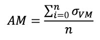 Equation 1
Instead of using the arithmetic mean, and following the idea presented by Dumont et al. (2005), we used a weighted mean: the Mesh-Weighted Arithmetic Mean (MWAM). For the MWAM some data points contribute more than others depending on the size of the element. This corresponds to the sum of the value of the Von Mises stress for each element multiplied by its own area (A) and divided by the total area (Equation 2). In Equation 2, we demonstrate that this value is equivalent to the division of the arithmetic mean of the product of stress and area by the arithmetic mean of the area, which is easier to calculate and does not require the correction of the weight element by element.
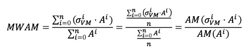 Equation 2
If all weights are equal, then the weighted mean is the same as the arithmetic mean. Therefore, in a uniform mesh, AM and MWAM will be the same.
Mesh-weighted median of stress distribution. The median is the middle measurement of any set of sorted data. That is to say, this statistic is the value of the data that has an equal number of items on either side of it, after arranging the data in order of magnitude (e.g., ranks) and divides a frequency distribution into two halves (Sokal and Rohlf, 1987). It is the middle order statistic when n is odd. When n is even, it is the average of the orders statistics with ranks (n/2) and (n/2) + 1 should be used (Rousseeuw and Croux, 1993). This statistic is useful as an estimator of central tendency, and is resistant to deviations from normality and the presence of outliers. In the case of FEA, the median would be the value separating the higher half from the lower half of the values of Von Mises stress recorded in each element of the mesh after they have been ordered.
Here the Mesh-Weighted Median (MWM) of stress distribution has been defined as the division of the median of the product of stress and area by the median of the area (Equation 3), based in the formulation presented in Equation 2.
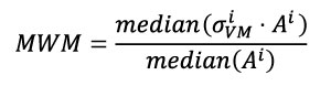 Equation 3
Evaluating the degree of homogeneity of the mesh. Although these corrected statistics can be used in a comparative analysis, they are limited to the main descriptive values in a set of data. The distribution of the data is also extremely useful information and is not captured by central tendency statistics. For example, two structures could have the same median value, but one could have more extreme values than the other. Biologically, that means that one specimen has areas with much higher stress than the other, which could be relevant information regarding the biomechanics of this structure. This difference would only be seen by comparing distributions. However, in comparing distributions, it is important to consider the size of the elements of the mesh.
Therefore, we propose two indicators to evaluate whether a mesh is uniform enough to use the raw stress data for statistical analysis: the Percentage Error of the Arithmetic Mean (PEofAM) and the Percentage Error of the Median (PEofM). These two indicators evaluate the difference between the non-weighted value and the weighted value of mean and median (PEofAM in Equation 4 and PEofM in Equation 5),
![]() Equation 4
Equation 4
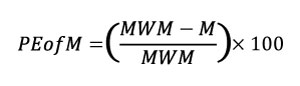 Equation 5
If the mesh of the model is close to an ideal fine uniform mesh, the non-weighted and the weighted indicators should be equal. If the error is lower than a certain threshold, the mesh can be considered an ideal mesh where all the elements have an equal weight. In this work we call those meshes Quasi-Ideal Meshes (QUIM) to avoid confusion with a true uniform mesh. When both values are similar, that mesh can be considered a QUIM, and quantitative and statistical analysis of the FEA data can be computed without any corrections. The validity of this approach has been evaluated using a lower mandible of Chlamyphorus truncatus, by varying the mesh uniformity and element size and computing the described statistics for each mesh.
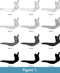 Evaluating different meshes. First, 12 different meshes (Figure 1) were created with the set of forces and boundary conditions described below, ranging from a coarse mesh to a fine mesh, following the procedure described by Bright and Rayfield (2011). In Finite Element mesh generation, this overall size of the elements does not mean that all the elements have exactly the same size, but the elements, whenever it is geometrically possible, have a similar size.
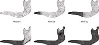
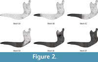
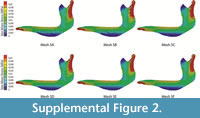
Second, a series of six different meshes of the same Chlamyphorus truncates mandible were also developed (Figure 2). In this case, the meshes varied from an absolutely non-uniform mesh to a mostly uniform mesh. The complexity of the geometry makes a perfect uniform mesh impossible.
All statistical values were calculated for each mesh in the series iteratively. That is, values were calculated for the first and second mesh, and a percent relative error (ε[%]) was calculated (Schmidt et al., 2009). Subsequently, values were calculated for the third mesh, and compared with the second using the same metric. This process continued for all meshes until the point where changing the size or uniformity of the mesh did not affect the outcome of the analysis. To analyse statistical convergence is a common procedure in FEA (Richmond, 2007; Tseng et al., 2011b; Tseng and Flynn, 2014). In order to reach an accurate solution, it is important to ensure that the FE model contains enough nodes, so the result does not change when the size of the mesh is decreased (Bright and Rayfield, 2011).
 It is important to note that (ε[%]) evaluates the convergence of the statistics prior to the reduction of the size of the elements of the mesh whereas PEofAM and PEofM are evaluating the difference between the statistics with and without the weighting of the mesh.
Case of Study: Ecomorphology of Cingulata’s Mandibles
Material. Twenty different mandibles belonging to 14 species of Cingulata have been analysed, three of which are extinct (Table 1). This material is housed in different museums (Table 1). Although we previously developed an FEA on these species (Serrano-Fochs et al., 2015), this time we add six new specimens in an effort to examine intraspecific variability.
FEA models. Plane models of the mandibles were created according to the methodology summarized by Fortuny et al. (Fortuny et al., 2012) using ANSYS FEA Package v.14.5 for Windows 7 (64-bit system) from two-dimensional geometries. The thickness of the model has been assumed constant in the mandible and obtained from the individual average of three measurements: mandibular width at the first jugal, mandibular width at half of the level of antero-posterior length of the jugal series and mandibular width at the posterior end of the jugal series. Von Mises stress distributions of the planar models were obtained for comparison.
Two main muscles (temporalis and masseter) were included in the model as force vector between the centroid of the muscular attachment in the lower mandible and the centroid of the equivalent muscle attachment in the skull (Serrano-Fochs et al., 2015). Following this direction, the force vector was applied in the insertion area of each muscle and because the amount of force that a muscle produces depends on the section of the muscle (Alexander, 1992), the force was applied to all the models in both muscles insertion areas (masseter and temporalis) and depending of the proportion of its insertion area described in Table 1.
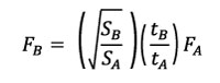
In order to compare the models, a scaling of the values of the forces was applied according to a quasi-homothetic transformation of the FE models (Marcé-Nogué et al., 2013) and following Equation 6. An arbitrary force of 1 N was applied to Chaetophractus villosus, which was the reference model for this study.
 Equation 6
where SA is the area of a reference model, SB the area of a scaled model, tA is the thickness of a reference model and tB the thickness of a scaled model.
Data for the Cingulate species used in this study regarding: the area of the lower mandible, insertion places, forces (musculature applied force per unit area [N/mm2]), and the thickness and scale factor variables used in the quasi-homothetic transformation are described in Table 1.
The boundary conditions were defined and placed representing the loads, displacements and constraining anchors that the structure experiences during function as in previous works (Serrano-Fochs et al., 2015). They simulate the mandible constrained at the most anterior part and a constraint on the condyle at the level of the mandibular notch representing the immobilization of the mandible.
A mesh of quadrilateral elements was created for each model. Isotropic and linear elastic properties were assumed for the bone. In the absence of data for Cingulata or any close relative, or any mammal clade with similar bone structure, the mandible properties of Macaca mulatta was used: E (Elasticity Modulus) = 21,000 MPa and v (Poisson coefficient) = 0.45 (Dechow and Hylander, 2000). The choice of this taxon it is due to its ecological history and is discussed in Serrano-Fochs et al. (2015), although in a comparative analysis, these material properties are not relevant in the results of stress (Gil et al., 2015). The data obtained in the FEA will be the Von Mises stress distribution which, according to Doblaré et al. (2004), is the most accurate variable to predict stresses when isotropic properties with a cortical bone as a material are used.
Comparative analysis and statistics. As mentioned above, the proposed approach was applied to the stress value of the FE results of the Cingulata mandibles. Our null hypothesis was that there would be no differences in stress values between different diets; thus, species were categorized by diet (Table 1). For some species more than one specimen (i.e., different lower jaws belonging to different individuals) were included.
To analyse the distribution and median values of the stress for the different mandibles, box-plots were used. The box-plot is depicted as a box where the upper and lower ends represent 25 and 75 quartiles, while the horizontal line crossing the box corresponds to the median (Quinn and Keough, 2002). In this case the lines extending up and down the box (called whiskers) included 80% of the values. This way to represent the stress distribution follows the idea of Dumont et al. (2005), Parr et al. (2012) or Figueirido et al. (2014) to represent it via frequency plots but facilitates the comparison between models and includes the corrections to account for the uniformity of the mesh. On this line to standardize the mesh to remove the effect of the non-homogeneity, the work of Tseng (2008) proposed an alteration in the values of each element with a correction based in the median values of the size of the element. The methodology proposed avoids the alteration of the results of each element of the mesh using the evaluator QUIM to certify that the mesh can be used or not for statistical metrics.
Normality of the stress values for each specimen was checked with a Shapiro-Wilks test (Table 2). In order to see if there were differences in stress values between different diets, a Kruskal-Wallis test was applied to the weighted median values of each specimen; Medians were used instead of means because stress distributions were not normally distributed. Kruskal-Wallis tests the null hypothesis that there is no differences between groups and is based on ranking the pooled data (Quinn and Keough, 2002). Although they were included in the graphical representations, herbivorous species were not included in the statistical analysis because they were represented by only two extinct species, and one of them belongs to a different taxonomic group from armadillos (Vassalia maxima, Pampatheriidae).
RESULTS
Evaluating the Size and the Homogeneity of the mesh: Finding the Quasi-Ideal Mesh
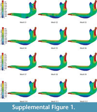 The Von Mises Stress distributions for the 12 different meshes with decreasing mesh size of a Chlamyphorus truncatus mandible are shown at Figure S1. The proposed statistics for each mesh and the values of the percent relative error in the convergence of the meshes are summarised in Table S1 and Table S2.
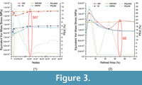
The different types of mesh created for Chlamyphorus truncatus mandible showed that the values of the statistics AM, M, MWAM and MWM vary for coarse meshes, and tend to converge on a specific value whenever the meshes are finer (Figure 3.1). This result is reinforced with the percent relative error (ε[%]), which has a tendency to reduce the value for each statistic (Figure 4.1).
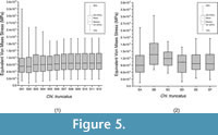
The relationship between the weight-meshed values with their relative non-weighted values was evaluated with the PEofAM and PEofM. Although smaller values can be obtained, at 2% of PEofAM and 5% of PEofM, the MWAM and MWM converge (i.e., their values do not change despite having meshes with smaller elements, and the percent relative error is small). Moreover, the distributions of these meshes (Mesh S07 from Figure 5.1) were also stabilized in relation to the mesh variation. We considered a value to be stabilized when the differences between the previous and the next iterations are small.
 Therefore, this is the threshold that can be used as optimal for obtaining the QUIM in this case. We can assume for a general case that the first mesh that achieves those error values or smaller can be considered to be the QUIM.
The proposed statistics were also evaluated in regards to the degree of homogeneity of the mesh. The Von Mises stress distribution of the six different meshes of Chlamyphorus truncatus are shown in Figure S2, and their values are summa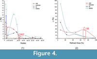 rised in Table S3 and Table S4.
The variation of the statistics AM, M and MWM for mesh homogeneity was greater than in the first case, when we studied the size of the mesh. They reached convergence when the mesh was practically uniform (Figure 3.2 and Figure 4.2 for the percent relative error). Despite this, MWAM had an almost constant value for all the meshes, regardless of mesh homogeneity.
PEofAM and PEofM have the smallest differences between mesh-weighted and non-mesh weighted values when the meshes are practically homogenous. Moreover, the box-plots for these meshes have a similar distribution at 70% of mesh uniformity (mesh SE of Figure 5.2). That mesh is the same proposed as QUIM following the threshold of 2% of PEofAM and 5% of PEofM. It means that the threshold used as optimal for obtaining the QUIM can be adopted regarding the uniformity of the mesh, too.
Case Study: Ecomorphology of Armadillo Lower Mandibles
 Two percent for PEofAM and 5% for PEofM were used in order to obtain the QUIM for each armadillo mandible. There were only small differences between non-weighted and mesh-weighted statistics for this mesh. Table 3 indicates the number of nodes for each model
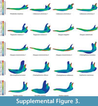
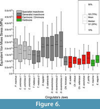 for each QUIM. The maps of the Von Mises Stress distribution of all of the mandibles herein analysed can be found in Figure S3.
Descriptive statistics AM, M, MWAM, MWM, PEofAM and PEofM are summarized in Table 3 for all the cingulate mandibles. Kruskal-Wallis test showed statistical differences between omnivores, and both groups of insectivores have been found (Table 3).
From the box-plots, it is clear that insectivorous species have larger median stress values and a larger spread of data (Figure 6). Herbivores have a range of values quite similar to carnivores, while insectivores have larger mean and median values in general.
DISCUSSION
Convergence of the Values When Modifying the Mesh
 Varying the size of the elements of the mesh. The convergence of AM, M, MWAM and MWM values agrees with the previously published works in that it is necessary to use small mesh elements to obtain accurate results (Bright and Rayfield, 2011; Tseng and Flynn, 2014). Following our results with Chlamyphorus truncatus, when the meshes are composed by less than 25,000 nodes (Figure 3.1), the arithmetic mean (AM) showed different values. However, up to this number of nodes, the value of AM for different meshes converged. Therefore, as AM converged at 25,000 nodes we can consider this mesh as having elements small enough for a statistical analysis without any further correction. As for the AM, the non-weighted median (M) had different values for meshes composed by less than 25,000 nodes (Figure 3.1). Up to this number of nodes, the value of M converged (i.e., it was very similar despite having smaller elements).
On the other hand, the weighted value (MWAM) converged with less than 1,000 nodes (Figure 3.1). This means that MWAM is more resistant to changes in the size of the elements of a mesh and should be used instead to compare different models independently of mesh size. Unlike the MWAM, the weighted median (MWM) behaved similarly to the median and had a similar point of convergence. This means that the MWM will not correct errors due to different sizes of the element of the mesh.
 Varying the degree of homogeneity of the mesh. Although most FE studies actually include more uniform models than those tested here, it is important to be aware of the effect of non-uniform meshes. Considering mesh uniformity, convergence of the values AM and MWAM is reached when the mesh is practically homogeneous (Figure 3.2). When the mesh is not homogeneous, AM varied greatly whereas MWAM was practically constant when varying the homogeneity of the mesh. This means that MWAM is more independent of the degree of homogeneity of the mesh than AM.
On the other hand, M and MWM behaved similarly when meshes were non-uniform, reaching a consistent value for percent relative error when meshes were mostly homogenous (Figure 4.2). Although MWM does not correct the non-uniform problems, it is a value that helps us define the QUIM when calculating PEofM.
Differences Between Mesh-weighted and Non-weighted Statistics: Percentage Errors
When the different meshes of Chlamyphorus truncates were analysed, important differences between the mesh-weighted and the non-weighted statistics were obtained for the same mesh. The greatest differences were in PEofAM and PEofM in the coarsest meshes; these differences were smaller when the mesh was finer (Figure 3.1 when the size of the elements is reduced and Figure 3.2 when the mesh reaches homogeneity).
However, there is a relationship between the convergence of the mesh and the reduction of the differences between the mesh-weighted and the non-weighted values evaluated in PEofAM and PEofM although they are two absolutely different concepts that must be studied separately. In fact, PEofAM and PEofM are values that also converge when reducing the size of the elements and when reaching the homogeneity (Figure 3).
Taking into account this relationship between convergence (evaluated via ε[%]) and difference between weighted and non-weighted statistics (evaluated via PEofAM and PEofM), when the size of the elements of the mesh reached the converged value for the mean (M) of Von Mises stress, PEofAM is lower than 1% and PEofM is around 5% (Figure 3.1). Moreover, when the uniformity of the mesh is analysed and the mesh reaches the median converged value of Von Mises stress (Figure 3.2), PEofM is lower than 1% and PEofAM is around 5% (Figure 3.2).Therefore, from a certain number of nodes, the values of M and MWM and the values of AM and MWAM can be assumed to be practically the same.
This suggests that PEofAM and PEofM are suitable indicators for correcting the effect of the size of the elements of the mesh as well as the effect of the non-uniformity. Therefore, they were used to define the QUIM: when PEofAM and PEofM are lower than our proposed threshold, the mesh can be considered as a statistically ideal mesh to evaluate the distribution of the data.
Distribution of Stress Values
When the size of the elements of the mesh is reduced in Chlamyphorus truncatus model, the distribution of the values converged. (Figure 5.1). The outliers below the lower whiskers are the places where the stresses are practically null. The upper outliers should not be considered because they are numerical singularities due to the presence of artificial high stress values at the points where the displacement boundary conditions are applied. As the elements get smaller, the artificial high stress values become higher (Dumont et al., 2009). Therefore, these extreme values cannot be stabilized in a final value by changing the mesh. On the other hand, 90% of the values of the stress distribution can be stabilized in its final value despite the variation of the size of the elements (80% inside the whiskers and the lower 10%) following the idea proposed in Walmsley et al. (2013), where the maximum value is not analysed for the presence of artefact values. For our example, Chlamyphorus truncatus, the stabilization of the values happened at around 25,000 nodes (Mesh S07 of the Figure 5.1). It is worth mentioning that this coincides with the number of elements where the mesh has a PEofM lower than 2% and PEofAM 5%, supporting the use of those indicators for chosen the QUIM. The distribution of stresses remained constant from 70% uniformity and above (mesh SE of Figure 5.2).
Comparisons among Different Cingulate Mandibles
The significant differences among different diets found in the statistical analyses were more conclusive than the results obtained when analysing stress values at specific points of the mandible (Serrano-Fochs et al., 2015), where no statistical differences were found. That supports the analysis of the stress values of the whole specimen more than just a few isolated points, or at least the use of both sources of information (as isolated points could give an alternative view at specific areas).
However, this significance should be interpreted as illustrative more than a specific p-value. This is because when a Bonferroni correction was applied the mean values between specialized insectivores and omnivores are non-significant (most probably due to the small sample size of the specialist insectivores). Also, specimens from the same species were included in the sample and no phylogenetic correction was made, so there is lack of independence between points (Felsenstein, 1985).
Independent of the statistical results, the distribution of the data is explanatory enough (Figure 6), indicating clear differences between omnivores and herbivores (with small median values and tight distributions) and both groups of insectivores, with wider distributions and larger median values of stress. The only exception is Chl. truncatus, which has values that are much more similar to omnivores than to insectivores. This agrees with previous results (see discussion about this species in Serrano-Fochs et al., 2015).
It is noteworthy than both specimens of T. matacus showed a similar pattern, supporting the use of only one individual per species for FEA analysis (the normal procedure in biology: Pierce et al., 2008; Fortuny et al., 2011; Piras et al., 2013; Serrano-Fochs et al., 2015; Tseng and Flynn, 2015). On the other hand, D. novemcinctus show a range of variability that includes the other species of the genera. Although in these cases only two specimens have been included, this is the first time than more than one specimen from the same species has been included in FEA. Our results suggest that intraspecific variability could be different in different species. However that requires further research including an appropriate sample with more specimens per species. All the mean values are higher than the median values, stressing the fact that very high values due to the numerical singularities that appear at the constraints behave as outliers.
CONCLUSIONS
Our proposed approach has been shown to be useful. The Mesh-Weighted Arithmetic Mean is a useful statistic mostly independent of the mesh characteristics, and it is the recommended central tendency statistic when the mesh properties are not evaluated. It gives more accurate results than the Arithmetic Mean. Conversely, the Mesh-Weighted Median does not produce improved results when compared with the Median in non-homogeneous meshes. Therefore, before comparing mean or median values of stress, distributions the homogeneity of the meshes should be addressed. If they are non-homogenous then the Mesh Weighted Arithmetic Mean should be used (MWAM) instead of a regular arithmetic mean. In particular, the methods proposed have been shown to be extremely useful when analysing the biomechanics of vertebrate bone structures that can be modelled as planar models in an interspecific comparative framework.
For the ecomorphological approach of the cingulate mandibles, MWAM, MWM and box-plots give a clear overview of the results from the Von Mises stress values for each mandible: insectivores have a much larger dispersion of Von Misses stress and higher MWAM and MWM values than herbivores and omnivores/carnivores. The use of a general stress value plus the analysis of the stress distribution produced more complete information that can be combined with the values of stress obtained at isolated points when analysing the biomechanics of a structure in a comparative framework.
Further work should analyse how to apply these methodologies to 3D models, as well as analyse the intraspecific variation of the species, in order to ensure that using a single specimen for FEA is representative of the overall biomechanics the studied species.
ACKNOWLEDGEMENTS
We would like to acknowledge to E. Westwig, M. Reguero, M. Merino and F. Mayer, who provided S.D.E.T. access to the collections and kindly help with us with the information about specimens. We deeply appreciate the help of M. Tallman with the English revision and for her comments that have improved the manuscript. This work was greatly improved with the reviews of one anonymous reviewer.
REFERENCES
Adams, D.C., Rohlf, F.J., and Slice, D.E. 2004. Geometric morphometrics: ten years of progress following the “revolution.” Italian Journal of Zoology, 71:5-16.
doi:10.1080/11250000409356545
Alexander, R.M. 1992. Exploring Biomechanics: Animals in Motion. Scientific American Library, New York.
Aquilina, P., Chamoli, U., Parr, W.C.H., Clausen, P.D., and Wroe, S. 2013. Finite element analysis of three patterns of internal fixation of fractures of the mandibular condyle. British Journal of Oral and Maxillofacial Surgery, 51:326-331.
doi:10.1016/j.bjoms.2012.08.007
Attard, M.R.G., Parr, W.C.H., Wilson, L.B., Archer, M., Hand, S.J., Rogers, T.L., and Wroe, S. 2014. Virtual reconstruction and prey size preference in the mid Cenozoic thylacinid, Nimbacinus dicksoni (Thylacinidae, Marsupialia). PLoS ONE, 9:e93088.
doi:10.1371/journal.pone.0093088
Benazzi, S., Nguyen, H.N., Kullmer, O., and Hublin, J.J. 2014. Exploring the biomechanics of taurodontism. Journal of Anatomy, 226:180-188.
doi:10.1111/joa.12260
Bright, J.A. and Rayfield, E.J. 2011. The response of cranial biomechanical finite element models to variations in mesh density. The Anatomical Record, 294:610-620.
doi:10.1002/ar.21358
Dechow, P.C. and Hylander, W.L. 2000. Elastic properties and masticatory bone stress in the macaque mandible. American Journal of Physical Anthropology, 112:553-574.
Degrange, F.J., Tambussi, C.P., Moreno, K., Witmer, L.M., and Wroe, S. 2010. Mechanical analysis of feeding behavior in the extinct “terror bird” Andalgalornis steulleti (Gruiformes: Phorusrhacidae). PLoS ONE, 5:e11856.
doi:10.1371/journal.pone.0011856
Doblaré, M., Garcı́a, J.M., and Gómez, M.J. 2004. Modelling bone tissue fracture and healing: a review. Engineering Fracture Mechanics, 71:1809-1840.
doi:10.1016/j.engfracmech.2003.08.003
Doyle, B.J., Callanan, A., Burke, P.E., Grace, P.A., Walsh, M.T., Vorp, D.A., and Mcgloughlin, T.M. 2009. Vessel asymmetry as an additional diagnostic tool in the assessment of abdominal aortic aneurysms. Journal of Vascular Surgery, 49:443-454.
doi:10.1016/j.jvs.2008.08.064
Dumont, E.R., Grosse, I.R., and Slater, G.J. 2009. Requirements for comparing the performance of finite element models of biological structures. Journal of Theoretical Biology, 256:96-103.
doi:10.1016/j.jtbi.2008.08.017
Dumont, E.R., Piccirillo, J., and Grosse, I.R. 2005. Finite-element analysis of biting behavior and bone stress in the facial skeletons of bats. The Anatomical Record Part A: Discoveries in Molecular, Cellular, and Evolutionary Biology, 283:319-330. doi:10.1002/ar.a.20165.
Felsenstein, J. 1985. Phylogenies and the comparative method. American Naturalist, 126:1-15.
doi:10.1086/284325
Figueirido, B., Tseng, Z.J., Serrano-Alarcón, F.J., Martín-Serra, A., and Pastor, J.F. 2014. Three-dimensional computer simulations of feeding behaviour in red and giant pandas relate skull biomechanics with dietary niche partitioning. Biology Letters, 10:20140196.
doi:10.1098/rsbl.2014.0196
Fish, J.F. and Stayton, C.T. 2014. Morphological and mechanical changes in juvenile red-eared slider turtle ( Trachemys scripta elegans) shells during ontogeny. Journal of Morphology, 275:391-397. doi:10.1002/jmor.20222
Fletcher, T.M., Janis, C.M., and Rayfield, E.J. 2010. Finite element analysis of ungulate jaws: can mode of digestive physiology be determined? Palaeontologia Electronica 13.3.21A: 1-13 palaeo-electronica.org/2010_3/234/index.html
Fortuny, J., Marcé-Nogué, J., De Esteban-Trivigno, S., Gil, L., and Galobart, À. 2011. Temnospondyli bite club: ecomorphological patterns of the most diverse group of early tetrapods. Journal of Evolutionary Biology, 24:2040-2054.
doi:10.1111/j.1420-9101.2011.02338.x
Fortuny, J., Marcé-Nogué, J., Gil, L., and Galobart, À. 2012. Skull mechanics and the evolutionary patterns of the otic notch closure in capitosaurs (Amphibia: Temnospondyli). The Anatomical Record, 295:1134-1146.
doi:10.1002/ar.22486
Fortuny, J., Marcé-Nogué, J., Heiss, E., Sanchez, M., Gil, L., and Galobart, À. 2015. 3D Bite Modeling and Feeding Mechanics of the Largest Living Amphibian, the Chinese Giant Salamander Andrias davidianus (Amphibia: Urodela). PLoS ONE, 10:e0121885.
doi:10.1371/journal.pone.0121885
Gil, L., Marcé-Nogué, J., and Sánchez, M. 2015. Insights into the controversy over materials data for the comparison of biomechanical performance in vertebrates. Palaeontologia Electronica 18.1.10A: 1-24 palaeo-electronica.org/content/2015/1095-controversy-in-materials-data
Gunz, P., Mitteroecker, P., Neubauer, S., Weber, G.W., and Bookstein, F.L. 2009. Principles for the virtual reconstruction of hominin crania. Journal of Human Evolution, 57:48-62.
doi:10.1016/j.jhevol.2009.04.004
Marcé-Nogué, J., DeMiguel, D., De Esteban-Trivigno, S., Fortuny, J., and Gil, L. 2013. Quasi-homothetic transformation for comparing the mechanical performance of planar models in biological research. Palaeontologia Electronica 16.3.6T: 1-15 palaeo-electronica.org/content/2013/468-quasihomothetic-transformationMarcé-Nogué, J., Fortuny, J., Gil, L., and Galobart, À. 2011. Using reverse engineering to reconstruct tetrapod skulls and analyse its feeding behaviour, paper 237. In Topping, B.H.V. and Y. Tsompanakis, Y. (eds.), Proceedings of Thirteenth International Conference of Civil, Structural and Environmental Engineering Computing, Civil-Comp Press, Stirlingshire.
Marcé-Nogué, J., Fortuny, J., Gil, L., and Sánchez, M. 2015. Improving mesh generation in Finite Element Analysis for functional morphology approaches. Spanish Journal of Palaeontology, 30:117-132.
McHenry, C.R., Wroe, S., Clausen, P.D., Moreno, K., and Cunningham, E. 2007. Supermodeled sabercat, predatory behavior in Smilodon fatalis revealed by high-resolution 3D computer simulation. Proceedings of the National Academy of Sciences, 104:16010-16015.
doi:10.1073/pnas.0706086104
Neenan, J.M., Ruta, M., Clack, J.A., and Rayfield, E.J. 2014. Feeding biomechanics in Acanthostega and across the fish-tetrapod transition. Proceedings of the Royal Society of London B: Biological Sciences, 281.1781:20132689. doi:10.1098/rspb.2013.2689
O’Higgins, P. and Milne, N. 2013. Applying geometric morphometrics to compare changes in size and shape arising from finite elements analyses. Hystrix, the Italian Journal of Mammalogy, 24:126-132.
doi:10.4404/hystrix-24.1-6284
Parr, W.C.H., Wroe, S., Chamoli, U., Richards, H.S., McCurry, M.R., Clausen, P.D., and McHenry, C.R. 2012. Toward integration of geometric morphometrics and computational biomechanics: new methods for 3D virtual reconstruction and quantitative analysis of Finite Element Models. Journal of Theoretical Biology, 301:1-14.
doi:10.1016/j.jtbi.2012.01.030
Pierce, S.E., Angielczyk, K.D., and Rayfield, E.J. 2008. Patterns of morphospace occupation and mechanical performance in extant crocodilian skulls: a combined geometric morphometric and finite element modeling approach. Journal of Morphology, 269:840-864. doi:10.1002/jmor.10627
Piras, P., Maiorino, L., Teresi, L., Meloro, C., Lucci, F., Kotsakis, T., and Raia, P. 2013. Bite of the cats: relationships between functional integration and mechanical performance as revealed by mandible geometry. Systematic Biology , 62:878-900.
doi:10.1093/sysbio/syt053
Quinn, G. and Keough, M. 2002. Experimental Design and Data Analysis for Biologists. Cambridge University Press, Cambridge.
Redford, K.H. 1985. Food habits of armadillos (Xenartha: Dasypodidae), p. 429-437. In Montgomery, G.G. (ed.), The Evolution and Ecology of Armadillos, Sloths, And Vermilinguas. Smithsonian, Washington D.C.
Richmond, B.G. 2007. Biomechanics of phalangeal curvature. Journal of Human Evolution, 53:678-690.
doi:10.1016/j.jhevol.2007.05.011
Rousseeuw, P. and Croux, C. 1993. Alternatives to the median absolute deviation. Journal of the American Statistical Association, 88:1273-1283.
Schmidt, H., Alber, T., Wehner, T., Blakytny, R., and Wilke, H.J. 2009. Discretization error when using finite element models: analysis and evaluation of an underestimated problem. Journal of Biomechanics, 42:1926-1934.
doi:10.1016/j.jbiomech.2009.05.005
Serrano-Fochs, S., De Esteban-Trivigno, S., Marcé-Nogué, J., Fortuny, J., and Fariña, R.A. 2015. Finite element analysis of the Cingulata jaw: an ecomorphological approach to armadillo’s diets. PLoS ONE, 10:e0120653.
doi:10.1371/journal.pone.0120653
Sokal, R. and Rohlf, F. 1987. Introduction to Biostatistics . Dover Publications, Mincola, New York.
Topping, B.H.V., Muylle, J., Iványi, P., Putanowicz, R., and Cheng, B. 2004. Finite Element Mesh Generation. Saxe‐Coburg Publications, Stirling, UK.
Tseng, Z.J. 2008. Cranial function in a late Miocene Dinocrocuta gigantea (Mammalia: Carnivora) revealed by comparative finite element analysis. Biological Journal of the Linnean Society, 96:51-67.
Tseng, Z.J., Antón, M., and Salesa. M.J. 2011a. The evolution of the bone-cracking model in carnivorans: cranial functional morphology of the Plio-Pleistocene cursorial hyaenid Chasmaporthetes lunensis (Mammalia: Carnivora). Paleobiology, 37:140-156.
Tseng, Z.J. and Binder, W.J. 2010. Mandibular biomechanics of Crocuta crocuta, Canis lupus, and the late Miocene Dinocrocuta gigantea (Carnivora, Mammalia). Zoological Journal of the Linnean Society, 158:683-696.
Tseng, Z.J. and Flynn, J.J. 2014. Convergence analysis of a finite element skull model of Herpestes javanicus (Carnivora, Mammalia): implications for robust comparative inferences of biomechanical function. Journal of Theoretical Biology, 365:112-148.
doi:10.1016/j.jtbi.2014.10.002
Tseng, Z.J. and Flynn, J.J. 2015. Are cranial biomechanical simulation data linked to known diets in extant taxa? A method for applying diet-biomechanics linkage models to infer feeding capability of extinct species. PLoS ONE, 10:e0124020. doi:10.1371/journal.pone.0124020
Tseng, Z.J., Mcnitt-Gray, J.L., Flashner, H., Wang, X., and Enciso, R. 2011b. Model sensitivity and use of the comparative finite element method in mammalian mandible mechanics: mandible performance in the gray wolf. PLoS ONE, 6:e19171.
doi:10.1371/journal.pone.0019171
Vizcaíno, S.F. and Bargo, M.S. 1998. The masticatory apparatus of the armadillo Eutatus (Mammalia, Cingulata) and some allied genera: paleobiology and evolution. Paleobiology, 371-383.
Walmsley, C.W., Smits, P.D., Quayle, M.R., McCurry, M.R., Richards, H.S., Oldfield, C.C., Wroe, S., Clausen, P.D., and McHenry, C.R. 2013. Why the long face? The mechanics of mandibular symphysis proportions in crocodiles. PLoS ONE , 8:e53873.
doi: 10.1371/journal.pone.0053873
Wood, S.A., Strait, D.S., Dumont, E.R., Ross, C.F., and Grosse, I.R. 2011. The effects of modeling simplifications on craniofacial finite element models: the alveoli (tooth sockets) and periodontal ligaments. Journal of Biomechanics, 44:1831-1838.
doi:10.1016/j.jbiomech.2011.03.022
