Figure 1. The marine planktonic alga Calcidiscus leptoporus. The circular calcite platelets (coccoliths) are characterized by the diameter (yellow arrow) and the number of their sinuoidally shaped elements on their outer surface: Morphotypes within the Calcidiscus leptoporus-C. macintyrei plexus show moving clusters through geological time within the morphospace of diameter versus number of elements. Same specimen as illustrated in Knappertsbusch (2000) and Knappertsbusch (2001). The white scale bar at the upper border indicates 1 micrometer.
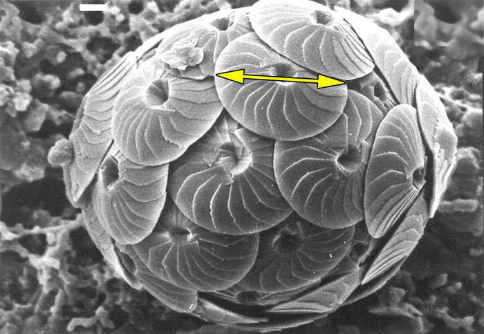
Figure 2. Stacked vertical slices through the density distribution model for C. leptoporus-C. macintyrei of Knappertsbusch (2000). The left panel shows color-coded stacks of near-baseline contours (2 specimens per grid-cell) of the model in "front view" (i.e., parallel to PCA I in figure 8 of Knappertsbusch, 2000). Slices are about 2 elements apart from each other. The uppermost slice (yellow to white) corresponds to the termination of the divergeing branch leading to morphotype D. The right panel shows color-coded stacks of near-baseline contours (2 specimens per grid-cell) in "side-view" (i.e., parallel to PCA II), at 1.02 units apart from each other (the slices correspond to those shown in figure 9 of Knappertsbusch, 2000). More than a decade ago this representation was the first view of the semi-continuous, four-dimensional hyperspace of the morphological variability in the C. leptoporus-C. macintyrei plexus. Though complicated, it gives an impression of the prominent divergence of extra-large coccoliths (morphotype D) between 12 Ma and 8 Ma.
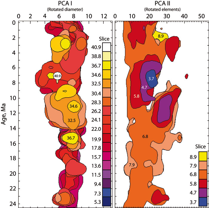
Figure 3. Globorotalia menardii in umbilical view. The calcitic shells of this planktonic foraminifer show considerable variation of the shell. Same specimen as illustrated in Knappertsbusch et al. (2009).
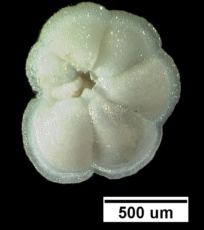
Figure 4. When seen in side view, globorotalid shells can be easily characterized by bivariate measurements of the spiral height (delta x) versus the length of the shell in keel view (delta y).
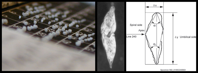
Figure 5. Flow-scheme of programs for the preparation of original data to a data model, that can be imported to Voxler for displaying frequency isosurfaces. See PDF version for zoomable version. Program names are written in bold and italics, input and output data are indicated in plane text.
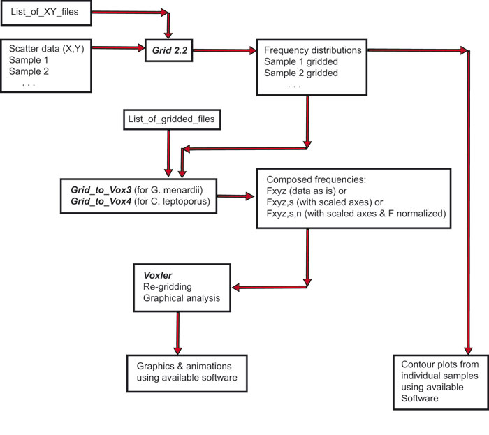
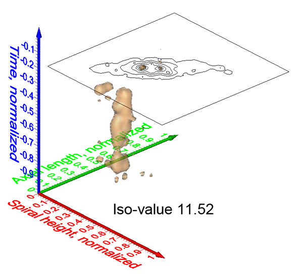
Figure 6. Steps from contoured bivariate data to interpolated iso-surfaces in the case of C. leptoporus. 1: Scatter plot of diameter versus elements from sample DSDP 251A-12-1, 88 cm. Grid-cells subdivide the diameter axis into intervals of 1 micrometer length and the diameter axis into intervals of 2 elements width. 2: Contoured absolute frequencies (see frequencies tabulated in Table 1 derived from scattered data shown in Figure 6.1 using the above grid-cell size of 1 micrometer x 2 elements). Contour intervals are 3 specimens per grid-cell. 3: Normalization of the axes. The center of each diameter interval is divided by 13.5 while the center of each element interval is divided by 53 (see text for further explanation). 4: A stack of contoured relative frequency distributions in the space of normalized diameter versus elements from three different geological times. The time axis is normalized by division of the age of each sample by the age of the oldest sample of the entire data set (i.e., 23.08 Ma). Between Figure 6.4 and Figure 6.5 absolute frequencies per sample were transformed into relative frequencies per sample. 5: Iso-surface after connecting outer contour lines of equal (relative) frequency throughout the complete set of C. leptoporus data. The illustrated iso-surface shows the evolution of rare coccoliths in the bivariate space of diameter versus number of elements. Increased frequencies of coccoliths are located inside the iso-surface. 6: Animated clips of the relative frequency iso-surface of C. leptoporus captured at changing stratigraphic levels (iso-surface values set to 1.52). Changing numbers in the lower right corner indicate the geological age in million years ago. To open an interactive animation please click here. Click here for viewing a flat, printable image series of the above animated scenes. The phylogenetic tree and positions of C. leptoporus-C. macintyrei morphotypes A, B, C, D, E, E', I, L and S (red letters) were taken from Knappertsbusch (2000) and projected into the animated iso-surface. Based on genetic evidence the extant morphotypes I and L are considered now as separate species Calcidiscus leptoporus and Calcidiscus quadriperforatus, respectively (Quinn et al., 2004), while the specific status of extant morphotype S is pending on documentation of its holococcolith bearing life-cycle phase (Quinn et al., 2003; Young et al., 2003).
PE NOTE: For opening this and the animations in the other figures, QuickTime Player should be installed for best performance.
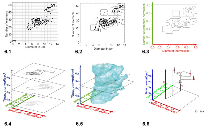
Figure 7. Steps from contoured bivariate data to interpolated iso-surfaces for G. menardii. 1: Scatter plot of spiral height versus axial width measurements (161 specimens) from sample DSDP 502A-1H-1, 15-20cm, which corresponds to the first sample in Figure 7 of Knappertsbusch (2007). 2: Contoured frequency plot of the data shown in Figure 7.1. delta X = 50 micrometers in X-direction and delta Y = 100 micrometers in Y-direction (see highlighted grid-cell in the lower left corner of Figure 7.1. Contour intervals are 2 specimens per grid-cell. Frequencies for this example are tabulated in Table 2. 3: Normalization of axes to unit values between 0 and 1. For this transformation the x-component (i.e., in direction of spiral height) of frequencies within each grid-cell was divided by 675 and by 1550 along the y-component (i.e., in direction of axial length). 4: A stack of contoured frequency diagrams from three different geological times. Notice that the time axis has been normalized to values between 0 and -1 by division of the age of each sample by the oldest sample age (8 Ma) of the data set described in Knappertsbusch (2007). Also, the absolute frequencies shown in Figure 7.2-3 were transformed into relative frequencies in Figure 7.4 for inter-sample comparison. 5: Iso-surface after connecting outer contour lines of equal relative frequency (isovalue of 1.28) throughout the complete set of G. menardii at DSDP Site 502A (Caribbean Sea). Frequent specimens are distributed inside the illustrated illustrated iso-surface, rare specimens are distributed towards the outer skin of the data body. 6: Animated clips of the relative frequency iso-surface of G. menardii at changing stratigraphic levels (iso-surface values set to 1.28) of DSDP Site 502A. Click here to open an interactive animation in a new window. Changing numbers in the lower right corner indicate the geological age in million years ago. 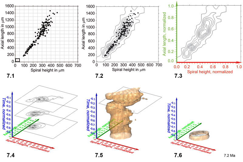
Figure 8. Spinning video animations of normalized density diagrams for a constant iso-value of 1.52 for C. leptoporus. All axes are normalized and represent diameter (red), number of elements (green) and time (blue). Click here 8.1, 8.2, and 8.3 to open and launch animations. 1 shows a solid iso-surface representation. Please notice the prominent and time-transgressive restriction of the density-surface (at about the level of the horizontal plane), which divides the model into a lower and an upper "valve." Click here for viewing a flat, printable image series of the animated scene of Figure 8.1. 2 shows the same iso-surface as in Figure 8.1 but in wireframe representation for a better visibility of the inserted phylogenetic tree. Click here for viewing a flat, printable image series of Figure 8.2. 3 illustrates the same data as shown in Figure 8.1, but as a wireframe diagram and spinning about a horizontal axis in order to show the iso-surface structure. Click here for viewing a flat, printable image series of Figure 8.3.
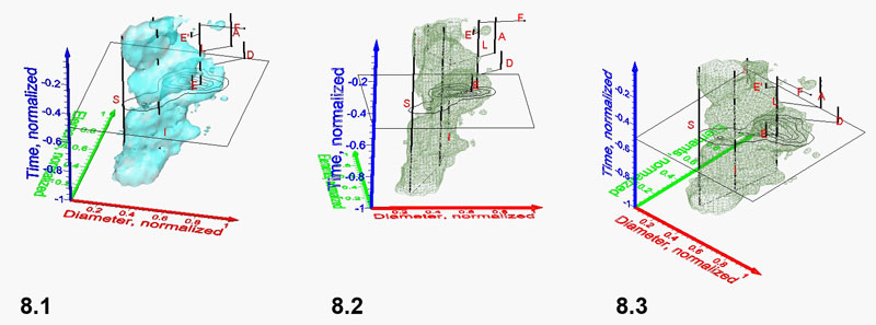
Figure 9.1-9.2 Spinning video animations of normalized density surface for G. menardii at Caribbean DSDP Site 502 (click here to launch animations 9.1 and 9.2. All axes are normalized and represent spiral height (red), axial length (green) and time (blue). Figure 9.1 shows a rotation cycle in counter-clockwise direction about a vertical spin-axis. A constant isovalue of 1.28 was selected to illustrate a low-frequency envelope of morphological trends through time in the spiral height versus axial length morphospace. Click here for viewing a flat, printable image series of Figure 9.1. Figure 9.2 shows the same iso-surface as in Figure 9.1 but rotating about a horizontal axis in direction towards the observer (click here for a printable, flat image series of the animated scene of Figure 9.2).
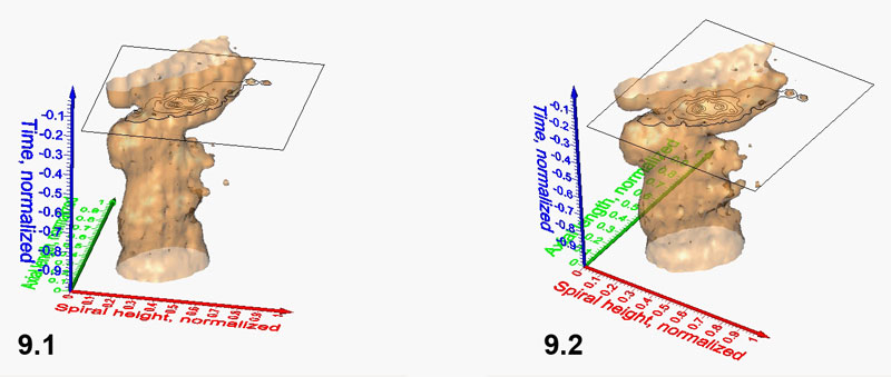
Figure 10.1-10.3. Iso-surfaces (isovalue=1.28) for G. menardii at the Caribbean DSDP Site 502 (Figure 10.1, which is the same model as shown in Figure 9) and DSDP Site 503 (Eastern Equatorial Pacific, Figure 10.2). Figure 10.3 shows involved iso-surfaces for both sites. Click here to launch animation of 10.3.
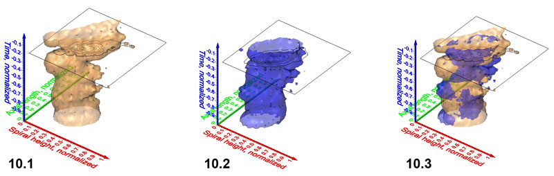
Figure 11.1-11.4. Frequency iso-surfaces for C. leptoporus coccoliths captured at increasing isovalues of 0.50 (Figure 11.1), 1.52 (Figure 11.2; same value as in Figure 8), 2.50 (Figure 11.3) and 4.00 (Figure 11.4). Axes are the same as in Figure 8.
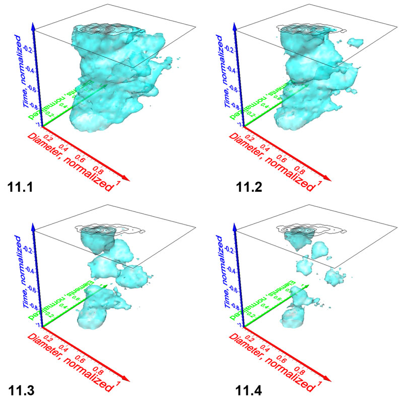
Figure 12.1-12.2. Pulsating diagrams of C. leptoporus in side view showing maximum coccolith variability (Figure 12.1) and in front view (Figure 12.2), where coccolith variability appears minimal. Axes are the same as in Figure 8. Click here to launch 12.1 and 12.2 animations. The projected phylogenetic dendrogram is the same as illustrated and discussed in Knappertsbusch (2000) and Knappertsbusch (2001). Numbers in the lower right corner of each animation indicate iso-value steps of 0.5.
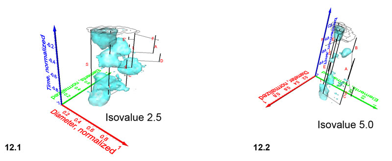
Figure 13.1-12.4. Iso-surfaces for frequencies of G. menardii at DSDP Site 502 taken at isovalues (normalized specimen densities) of 1.28, 4.90, 7.00 and 9.15, respectively. Axis names are the same as in Figure 9. The iso-surface for the value of 1.28 is also shown in the spinning diagrams in Figure 9.1 and 9.2.
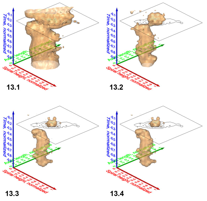
Figure 14. Animated sequence of frequency iso-surfaces for G. menardii at DSDP Site 502. Axis names are the same as in Figure 9. Click here to launch animation in a new window. Numbers in the lower right corner of the animation indicate iso-values at intervals of 1.28.