PAST - Case study 1 - The Permian brachiopod Dielasma

Case study 1 - The Permian brachiopod Dielasma from the north of England

The Permian brachiopod Dielasma is common at many localities within the Zechstein reef facies of the Ford Formation in the Sunderland area, N.E. England (Hollingworth & Pettigrew 1988). The smooth terebratulide brachiopod often forms monospecific clusters which are presumed to represent living assemblages at the base and within the reef. Large, well-preserved samples of the genus are available and a number of variates may be easily measured on complete specimens. Hollingworth & Pettigrew (1988) assessed the population structures and dynamics of a number of discrete populations of Dielasma in terms of salinity and other possible environmental fluctuations. Study of several samples suggest some populations were stunted; moreover it is possible that several subspecies or even species may be represented in the samples associated with the Permian reef.

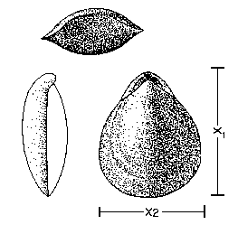
Two measurements were made, using vernier calipers, on three discrete samples of the terebratulide brachiopod Dielasma from the Ford Formation: the sagittal length (X1) and maximum width (X2) of the pedicle valve were taken on conjoined pairs. Data from three different sites (L1, L2 and L3) are available for analysis. With the information available it should be possible to compare and contrast the population structures and dynamics of each sample and moreover compare the relative outlines of the shells from all three localities. The data from all three localities are available on the file dielasma.dat.

Viewing the data

Open the file and select the column 'L1/X1'. Choose 'Histogram' in the Plot menu. In the same way, look at the L2/X1 and L3/X1 columns. If you are comparing graphs from a number of different data sets it may be useful to standardise your output with a uniform choice of start and end values for binning, and X and Y start and end values.

Also plot survivorship curves. How do these work?

The graphs for all three data files have different shapes. Why apparently are no minute growth stages represented in any of the samples? Account for the bimodal peaks manifest in the L1 data set. In marked contrast, L2 has a strong unimodal peak, with apparent high infant mortality, whereas L3 is trimodal. Explain!

More information about the plotting functions can be found in the manual.

Statistical tests

We will now formally test whether any of the variates are normally distributed. Select one X1 column at a time, and choose the Chi-square or the Shapiro-Wilk test depending on the sample size. Are the results in accordance with expectation from the visual inspection?

Also compare the X1 values from the different localities using the F and t tests, the Kolmogorov-Smirnov test or the Mann-Whitney U test as appropriate.

Regression and growth rates

For each locality, try to fit straight lines to the X1/X2 values ('Linear' in the Model menu). Use the RMA (Reduced Major Axis) method, and have both axes log-transformed. If the slope, a, does not differ significantly from 1 there are no apparent allometric effects, and it is more appropriate to plot using non-transformed axes. For each locality, assess the suitability of either the allometric or isometric growth equation, and write down the values for a and the standard error of a (we will use these below).

More information about linear regression can be found in the manual.

Comparison of growth rates

Are there significant differences in the growth rates of all three samples from different parts of the reef complex? Statistically significant differences in one such attribute, for example the growth rate between two variates, are often accorded subspecific status by taxonomists. For example, compare the isometric curve for X1 and X2 at locality L1 with the one at locality L2, by selecting 'F and t from parameters' in the Statistics menu and entering the respective values for a and the variance (square of standard error) of a. Do the growth rates differ from each other?

Professor William King first monographed these brachiopods on 1850 and established several subspecies of Dielasma. Do your analyses support King's observations?