| Case study 12 - Diversity through the Phanerozoic |
Data file: fr2.dat
The file is taken from the Fossil Record database at http://palaeo.gly.bris.ac.uk/frwhole/FR2.html (Benton 1993), and contains a summary of originations, extinctions, taxon richness and rates, for families of organisms through the whole of Earth's history. For a full explanation, see here.
Now move the Extinctions column (EXT) to column 2, next to the Time column, by dragging the column label. Select the first two columns (by clicking on TIME and then shift-clicking on EXT), and choose 'XY graph' in the Plot menu. Note the P-T and K-T extinction events.
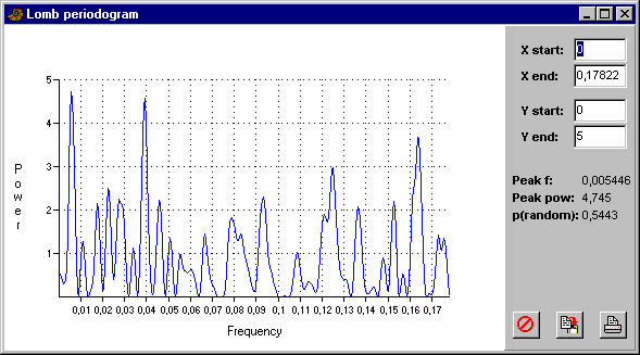
Now choose 'Spectral analysis' in the Time menu. Here is the result:

The 'Frequency' axis is in units of 1/(million years). The largest peak is placed at f=0.00545, corresponding to a period of 184 million years ('period' here meaning the time interval corresponding to one cycle). Since we are analyzing only 250 million years, we cannot have much confidence in this value (several periods should be included in the data). But the next highest peak is found at approximately f=0.039. This corresponds to about 26 million years - the 'Period of Doom' of Raup & Sepkoski (1984).
The hypothesis that the 184 myr peak results from a random sequence can not be rejected at p=0.1, and the 26 myr peak is even less prominent. However, these p values are relatively conservative, and the peak looks "convincing".
Try the same procedure on some of the other columns of data, for example the E/DT column (extinctions per diversity and time). Also try to analyze the EXT column with longer or shorter time ranges. You may find that the 26 myr cycle is difficult to reproduce, which indicates that the periodicity theory is less than robust.
More information about the spectral analysis module can be found in the manual.
The 'Autocorrelation' module would be interesting to try, but it cannot be used when the data points are unevenly sampled as in this case.
Open the file fr2.dat again, and commatize if necessary. Remove the Precambrian (PRE) row (select row and Cut), and then the KAS to HOL rows. This leaves the Vendian to Moscovian (Carboniferous). We leave out the Permian, because it is not fitted well by the logistic model (this may not be a very scientific procedure!). Now move the DIV (diversity) column to column 2, next to the TIME column. Select the first two columns, and choose 'XY graph' to visualize the data.
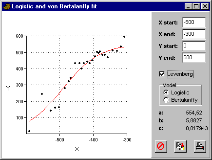
Next, choose 'Logistic' in the Model menu. Clicking the 'Levenberg' box will give a slightly better fit. The logistic equation that best fits the data is y=555/(1+5.9*exp(-5.1x)), where x is normalized to the range 0 to 1:

Is the logistic equation a good model? Compare with a linear model ('Linear' in the Model menu). It should be added that the logistic shape of the curve would have been more convincing if we had included only marine taxa in the analysis.
More information about the logistic fitting module can be found in the manual.
Open the file fr2.dat again, and commatize if necessary. Select the first 34 rows, from PRE to UFI (inclusive), and Cut (in the Edit menu, or using Ctrl-X). This leaves the Kazanian (Permian) to Recent.
Move the DIV (diversity) column to column 2, next to the TIME column. Select the first two columns, and choose 'XY graph' to visualize the data.
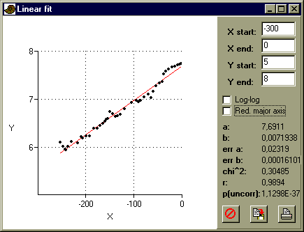
We will try to fit an exponential model to the data. PAST does not have a function for doing this directly, so we will take the logarithm and then fit to a straight line. Select the DIV column, and choose 'Log' in the Massage menu. Then choose 'Linear' in the Model menu:

The fit is almost perfect.
More information about the linear fitting module can be found in the manual.