METHODS
The ammonite specimens used to make the Coilopoceras springeri template, as well those used to evaluate the model, are from the National Museum of Natural History in Washington, D.C., the University of Texas Memorial Museum in Austin, Texas, various literature sources
(Table 1), and two field localities from the Chispa Summit Formation in Texas where over 80 unknown ammonite specimens were collected.
ArcGIS Desktop® 8.2 by ESRI was chosen for this project because of its spatial and database capabilities
(ArcGIS), and the easy point and click version (Desktop). Within the ArcGIS Desktop® software package, ArcInfo Workstation,
ArcMap, and ArcToolbox were utilized. Arc handles the spatial features (locations and shapes of objects), and Info handles the object's descriptions and how they relate to each other. The spatial information is the suture pattern. The database has information on each specimen of ammonite, such as its species name, catalog number, the suture length, and area of the sutural template.
To create the Coilopoceras springeri templates, suture patterns available in the literature were used. Important factors in the choice of using published information rather than original specimens are their accessibility. Ten
Coilopoceras springeri suture patterns (taken from 73 to 400 mm diameters) were scanned from publications and converted to a digital format.
Table 1 lists the 10 specimens, museum catalog numbers, and publications from which the suture patterns were obtained.
To test the accuracy of the Coilopoceras springeri templates, the suture patterns from museum specimens were traced directly from the specimen onto a transparency film, including both left and right shell sides. Suture patterns closest to the aperture were chosen to get the most complex pattern. Using a transparency to trace the sutures was an accurate transfer method and provided the capability to visualize the suture pattern clearly while tracing. It was also an efficient way to obtain a suture pattern for entry into the GIS. (For complete, step-by-step instructions of how to build a sutural template, see
Manship
2003).
The images were then scanned into Adobe Photoshop® 4 using a Hewlett-Packard Precision Scanner. In general, images are stored as raster datasets using binary or integer values and are positioned in some type of coordinate space. The suture images needed to be enlarged to be visible in
ArcEdit, so a width of 5,000 pixels was set for each suture pattern in Adobe Photoshop® 4. The images were also changed in Adobe Photoshop® 4 to grayscale (not RGB color). This change prevents the images from becoming a band of three colors
(RGB) when later converting from image to grid. Images were saved in the TIFF format, which is compatible with ArcInfo and ArcGIS Desktop®.
The suture images were next converted from the TIFF format to an ArcInfo grid
(ArcScan's primary raster data format). The grid places coordinates on the suture patterns, which is important for controlling scale and orientation. Scanned images are in a non-real world coordinate system (image space) and must be converted into some type of projection using x, y coordinates. The conversion is completed via ArcToolbox from ArcGIS Desktop®.
The grid-formatted suture patterns were opened using ArcTools through the ArcEdit environment. In order for ArcScan to capture the suture patterns, the grids must be converted into coverages for tracing. Coverages are file-based vector data storage formats used for storing attributes, projections, and shapes and are the primary vector format for ArcInfo and ArcGIS Desktop. The coverages store features such as arcs, polygons, tics, and links.
Each suture was digitized in ArcTools, using ArcEdit's editing environment. The process of digitizing converts features to a digital format using x, y coordinates. The coordinates were automatically recorded by the program and stored as spatial data. Manual adjustments were then performed, if necessary, to ensure an accurate tracing. Once the initial parameters were set correctly, automatic tracing proved efficient.
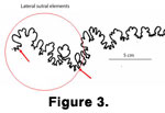 Once digitizing was complete, two tics (control points) were manually placed on predetermined positions on each suture pattern to allow the various sutures to be synchronized when aligning the patterns. The positions chosen for the tics were the beginning of the lateral saddle and the ending of the lateral lobe
(Figure 3). These positions were chosen to bound the lateral sutural elements, the area of maximum variation within the suture pattern. Because of its variability, this region is most useful for species recognition.
Once digitizing was complete, two tics (control points) were manually placed on predetermined positions on each suture pattern to allow the various sutures to be synchronized when aligning the patterns. The positions chosen for the tics were the beginning of the lateral saddle and the ending of the lateral lobe
(Figure 3). These positions were chosen to bound the lateral sutural elements, the area of maximum variation within the suture pattern. Because of its variability, this region is most useful for species recognition.
In the attribute table of the suture pattern
coverages, specimen identification columns were added. Attribute tables are tabular files containing rows and columns. Columns represent one attribute of a feature (or information describing the feature), such as the area of the polygon, length of the suture, or specimen identification. The rows represent the actual values and sutural pattern identifications. The species name and museum catalog numbers were inserted into the appropriate attribute table columns.
The Coilopoceras springeri suture pattern coverages must be converted from their coordinate system to a predefined coordinate system, so they will all overlay in the same orientation. The
Coilopoceras springeri holotype was chosen, combining opposing sutures from both left and right sides of the ammonite, for the basal suture pattern or destination. The left sutures were rotated in Adobe Photoshop® 4 to superimpose them with right sutures. The coverages of the other sutures (source) have been aligned or shifted to best fit the base pattern defined by the holotype (destination) using geometric transformations. The similarity transformation function compares and aligns the coordinates of the control points (the tics that were placed previously) and transforms the coverages to the new destination locations, keeping the aspect ratio of the suture patterns the same. This method scales all the sutures to the same size.
Once all the Coilopoceras springeri template sutures were transformed to the same destination locations or coordinates, they were merged together through the geoprocessing function. This process overlays coverage selections and performs analysis, topology processing, and data conversion. The output results from this operation created one layer of all 10
Coilopoceras springeri suture patterns merged, as well as their attribute tables, making the completed right/left template.
When the Coilopoceras suture patterns were merged together, they were changed into a
shapefile. Shapefiles are vector data storage formats, but to get correct topology, shapefiles must be converted back into
coverages. Topology in coverages refers to spatial relationships between connecting or adjacent features, arcs (sets of connected points), and areas (sets of connected arcs). Topology was created using the Clean and Build tools. Clean also corrected undershoots (an arc that does not extend far enough to intersect another arc) and overshoots (portion of an arc digitized past its intersection with another arc) within a specified tolerance, and placed nodes at each intersection. Manual editing was also used to correct small undershoots. Build was used to create a feature attribute table for the polygons. Dissolving the arcs within the polygon to make one polygon, based on specific attributes, was the last step.
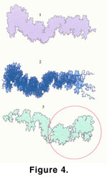 The completed Coilopoceras springeri
right/left template
(Figure 4.1) is an outer boundary of all the suture patterns used
(Figure 4.2) to make the polygon. To create the
right/left template, the Left
Coilopoceras springeri template (Figure
4.3) was reversed, aligning the tics with the original right Coilopoceras springeri
template.
Hoplitoides sandovalensis and Coilopoceras colleti templates were also made and tested in the same manner as stated previously. Recall that most variation in the suture pattern occurs within the lateral sutural elements. With only two tie points or tics added to each specimen, accuracy in overlaying the sutures is lost in the polygon beyond the second tic
(Figure 3 and Figure
4.3).
The completed Coilopoceras springeri
right/left template
(Figure 4.1) is an outer boundary of all the suture patterns used
(Figure 4.2) to make the polygon. To create the
right/left template, the Left
Coilopoceras springeri template (Figure
4.3) was reversed, aligning the tics with the original right Coilopoceras springeri
template.
Hoplitoides sandovalensis and Coilopoceras colleti templates were also made and tested in the same manner as stated previously. Recall that most variation in the suture pattern occurs within the lateral sutural elements. With only two tie points or tics added to each specimen, accuracy in overlaying the sutures is lost in the polygon beyond the second tic
(Figure 3 and Figure
4.3).
One quantitative method to compare the sutures tested within a template was to calculate the percentage of suture pattern length that did not fit within the template. This method used x-tools, a script downloaded from the
ESRI website. The Erase command removes the portion of the suture that falls within the template, leaving the bits of suture that fall outside of the template. This outside length can then be divided by the total suture line length to determine the percentage of suture length that falls outside of a template.
In another effort to quantitatively compare sutures, two sutures were compared against each other. The sutures were overlain and the area (polygon) between the two sutures was calculated. The GIS software automatically calculates the area of a polygon, allowing an easy and quantitative comparison of two suture patterns.
