EXAMPLE 2: BIODIVERSITY AND PALAEOENVIRONMENTAL INTERPOLATED BIOGEOGRAPHIC MAPS OF EUROPEAN NEOGENE LARGE LAND
MAMMAL FAUNAS
The following example shows how the Interactive Data Language can be used to model biodiversity and ecomorphologic proxies in the European Neogene geographic context.
The European continental Neogene has yielded hundreds of localities containing mammal remains. This important collection of data is now being used to study the evolution of biodiversity
(Fortelius et al. 1996,
Costeur et al. in
press) and palaeoecology of the mammalian communities (Fortelius et al. 1996,
Van Dam and Weltje 1999,
Fortelius et al. 2002,
Jernvall and Fortelius
2002). The different studies cited above have brought to light different large scale or regional patterns linked to climatic and/or geographic evolution in large or small mammal faunas. Our purpose here was twofold. First, we investigated the large mammal species geographic distribution in relation to the Neogene
palaeogeography. Second, we used ecomorphologic parameters to characterize large mammal communities on a taxon-free (Damuth
1992) ecological basis in order to infer past environments.
Palaeogeographic maps of the Neogene have been suggested
(Rögl 1999,
Meulenkamp and Sissingh
2003) but few biodiversity and/or palaeoecological studies have attempted to represent classical analysis results on maps. The IDL meta-language and its representation facilities offer the opportunity to investigate biogeographic and environmental patterns resulting from the analysis of mammalian communities with direct visualizations onto palaeogeographic maps.
Data
Two different datasets were used. The first was a collection of extant European large mammals (data from
Legendre 1989 and unpublished, and Héran unpublished), which was be used to test IDL interpolation functions. Comparisons of the results with recent studies on the distribution of land mammals
(Baquero and Telleria
2001) provided information on the reliability of the IDL tool.
The second dataset was a compilation of 100 Tortonian European localities that have yielded large fossil mammals
(Costeur unpublished). Their presence/absence as well as different ecomorphologic parameters (e.g.,
hypsodonty, tooth crown height) were recorded and evaluated. We used these to produce palaeobiogeographic maps of the distribution of species richness and of environmental proxies such as humidity/aridity. Palinspastic palaeogeographic backgrounds were built from published maps
(Rögl 1999,
Meulenkamp and Sissingh
2003), and their settings will be explained in the next section. Spatiotemporal coordinates for each locality were amalgamated from their ages and present-day latitude and longitude.
Algorithm
The algorithm used here was simpler than in the simulation of Triassic species richness. The algorithm was built in three steps.
Step One: Data Acquisition.
- Palaeogeographic maps were generated as before using Tortonian and Recent maps of Europe and North Africa. The first step was to load the map into a corresponding 60 x 100 binary matrix (zero for oceanic areas, one for continental areas; see
Figure 2 for an overview of the process). Each map covered the area between 30° North to 59.5° North and 10° West to 39.5° East. Each cell of the matrix thus represented an area of 0.5° x 0.5° corresponding to a mean surface of ca. 2200 km.
- Faunal data: Locality characteristics (palaeogeographic coordinates and values to be interpolated) were read by the program from a text file provided by the user.
Step Two: Interpolation.
Our program offers two interpolation methods from among those included in the IDL library: Delaunay triangulation and Thin Plate Spline
(TPS; Yu
2001). Sugihara and Inagaki (1995) described the Delaunay triangulation method. We will not discuss the mathematical foundations of these techniques here, but the basis for this interpolation method is to construct connected triangles between the data points and use them to determine unknown values by calculating a regression between their vertices. Thin Plate Splines apply a tight surface using a smooth bivariate function that takes the data points into account and assumes a minimum curvature of the surface
(Monnet et al.
2003).
Other interpolation methods exist, including the popular Kriging-Cokriging method
(Boer et al.
2001). Even though the Kriging algorithm is implemented as a routine in IDL, we did not use it because of the high subjectivity needed to choose the parameters that best fit the variogram, and because it is a computationally difficult method that requires an extensive practical experience compared to TPS and Delaunay triangulation.
TPS and Delaunay triangulation interpolate on a gridded geographic matrix so locality data provided by the user were placed in a matrix of the same dimensions as the palaeogeographic one (i.e., within cells of 0.5° x 0.5°). If more than one locality falls into the same cell, which is often the case with coarse resolution, several choices are proffered. Depending on the needs of the investigation, the minimum, maximum, mean, or median value of the parameter can be computed. The interpolation is then conducted on the matrix generated from the computed values. The computation does not distinguish coastal boundaries; a "continent" filter is later applied for visualization.
Step Three: Output.
A twofold sub-routine allows the validity of the results to be tested:
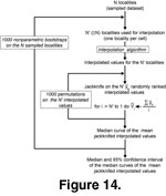 1. We first evaluated the "quality" of the interpolation results; for example, testing whether the dataset is large enough to yield a stable mean interpolated value regardless of the spatial distribution of the samples. To do this, we performed an analysis similar to a standard rarefaction procedure in which the relationship between the size of the set localities and the mean interpolated value was assessed. An algorithm involving three nested levels was applied
(Figure 14):
1. We first evaluated the "quality" of the interpolation results; for example, testing whether the dataset is large enough to yield a stable mean interpolated value regardless of the spatial distribution of the samples. To do this, we performed an analysis similar to a standard rarefaction procedure in which the relationship between the size of the set localities and the mean interpolated value was assessed. An algorithm involving three nested levels was applied
(Figure 14):
- The innermost level is a jackknife applied on the N' interpolated values associated with the sampled cells (N'
 N sampled localities because several sampled localities can be located in the same geographic cell). The resulting curve is made of N' mean interpolated values; it depends on the (arbitrary) order by which the N' interpolated values were successively
removed.
N sampled localities because several sampled localities can be located in the same geographic cell). The resulting curve is made of N' mean interpolated values; it depends on the (arbitrary) order by which the N' interpolated values were successively
removed.
- The second level was a random permutation of the N' interpolated values to randomize the removal order of the jackknife, which results in a median jackknifed curve which is independent of the removal order of the interpolated values, but still depends on the N sampled
values.
- The third level is a nonparametric bootstrap (random re-sampling with replacement) applied on the N sampled localities in order to estimate the median and confidence interval associated with the mean interpolated value parameter.
The resulting relationship (and its associated bootstrapped confidence interval) between the number of localities and the mean interpolated value strongly depends on the shape of the distribution of the interpolated variable, and thus illustrates an important statistical characteristic of the interpolation method that was
used.
 2. We then tested the reliability of the TPS-interpolated values by computing the correlation coefficient between observed and predicted values (
Monnet et al.
2003). This second test is obviously meaningless in the case of the Delaunay triangulation as the interpolated values for the sampled localities are the observed ones by definition of the method.
2. We then tested the reliability of the TPS-interpolated values by computing the correlation coefficient between observed and predicted values (
Monnet et al.
2003). This second test is obviously meaningless in the case of the Delaunay triangulation as the interpolated values for the sampled localities are the observed ones by definition of the method.
Results
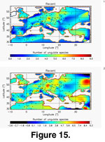
We tested the reliability of the IDL tool on the present-day distribution of large European mammal species richness. We interpolated species richness across Europe from 151 evenly distributed sampling points using Delaunay triangulation and TPS
(Figure 15).
Species richness is highest in Central Europe and decreases toward coastal areas as already demonstrated by
Baquero and Telleria
(2001). Those authors indicated that this pattern is consistent with a peninsular effect and decreasing land areas toward the borders as well as with the environmental parameters that prevail on the study area and the historical factors that affected Europe during the Quaternary. Both interpolation methods produced this same general pattern.
 We then investigated the link between present-day environmental variables and the distribution of species throughout Europe by means of direct comparisons between plots of morphologic characters related to the animals' ecology and plots of diverse environmental variables.
Such comparisons for present-day faunas would serve as a basis for relating large Neogene mammals to their environment.
We then investigated the link between present-day environmental variables and the distribution of species throughout Europe by means of direct comparisons between plots of morphologic characters related to the animals' ecology and plots of diverse environmental variables.
Such comparisons for present-day faunas would serve as a basis for relating large Neogene mammals to their environment.
Each species was assigned to a dental crown height class: brachydont (1), mesodont (2), or hypsodont (3) when their teeth possessed low, intermediate, or high crowns, respectively
(Fortelius et al.
2002). Each dental crown height class characterizes a particular type of diet, from one dominated by non-abrasive plants (mostly found in rather closed and humid environments) to one dominated by highly abrasive plants (mostly found in open and arid environments;
Fortelius and Solounias
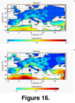
2000). 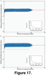 Mean dental crown height was calculated across species for each locality.
Figure 16 shows Delaunay triangulation and TPS interpolations of the present-day mean dental crown height values, and
Figure 17 and Figure
18 present the quality of the interpolation methods (note that the bootstrapped median jackknifed curves are shorter than the observed one due to random re-sampling of the same sampled localities reducing the number N' of geographic cells involved in the interpolation). For both methods the bootstrap median of the median jackknifed mean interpolated values, and their associated 95% confidence intervals were remarkably constant, even for small-sized datasets.
The negative bias that appeared with small-sized datasets (N' < 15 localities) is the logical consequence of the strongly right-skewed distribution of the mean hypsodonty values of the sampled localities. It is worth noting that the bootstrapped 95% confidence intervals estimated for the TPS method were wider than for the Delaunay triangulation method illustrating the greater sensitivity of the TPS algorithm to spatial heterogeneity of data.
Mean dental crown height was calculated across species for each locality.
Figure 16 shows Delaunay triangulation and TPS interpolations of the present-day mean dental crown height values, and
Figure 17 and Figure
18 present the quality of the interpolation methods (note that the bootstrapped median jackknifed curves are shorter than the observed one due to random re-sampling of the same sampled localities reducing the number N' of geographic cells involved in the interpolation). For both methods the bootstrap median of the median jackknifed mean interpolated values, and their associated 95% confidence intervals were remarkably constant, even for small-sized datasets.
The negative bias that appeared with small-sized datasets (N' < 15 localities) is the logical consequence of the strongly right-skewed distribution of the mean hypsodonty values of the sampled localities. It is worth noting that the bootstrapped 95% confidence intervals estimated for the TPS method were wider than for the Delaunay triangulation method illustrating the greater sensitivity of the TPS algorithm to spatial heterogeneity of data.
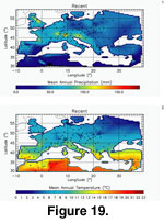
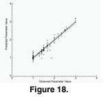 Figure 16 depicts a broad North/South gradient with a few areas of higher tooth crown height in eastern Spain, southern France, Switzerland, and northeastern Italy. If we directly compare this map to the present-day precipitation and temperature interpolated maps
(Delaunay Triangulation, Figure 19), we can associate the latitudinal differentiation with lower precipitation and higher temperature in the south, which is itself associated with more arid and open environments, thus explaining the hypsodonty maximum in that region. A multiple correlation analysis with temperature and precipitation as independent variables and hypsodonty as the dependent variable indicated a significant association: Pearson r = 0.522, bootstrapped (n = 10000) 99% Confidence Interval: 0.22 – 0.72; Mantel's t 0.0001 (n = 10000, H0 = no multi-linear association).
Figure 16 depicts a broad North/South gradient with a few areas of higher tooth crown height in eastern Spain, southern France, Switzerland, and northeastern Italy. If we directly compare this map to the present-day precipitation and temperature interpolated maps
(Delaunay Triangulation, Figure 19), we can associate the latitudinal differentiation with lower precipitation and higher temperature in the south, which is itself associated with more arid and open environments, thus explaining the hypsodonty maximum in that region. A multiple correlation analysis with temperature and precipitation as independent variables and hypsodonty as the dependent variable indicated a significant association: Pearson r = 0.522, bootstrapped (n = 10000) 99% Confidence Interval: 0.22 – 0.72; Mantel's t 0.0001 (n = 10000, H0 = no multi-linear association).
 Once the link between climatic parameters and ecomorphologic parameters such as mean hypsodonty has been characterized, it is possible to use that relationship to interpolate a similar map for fossil data. Here we present an example for the large Tortonian mammals (the other Neogene continental stages have also been investigated in the same way).
Figure 20 shows the hypsodonty pattern for 100 Tortonian sites distributed throughout Europe. We plotted the results onto a palaeogeographic map drawn from
Rögl (1999) using palaeo-coordinates calculated from present-day coordinates, as well as stratigraphic and geographic positions.
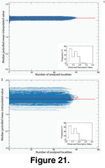
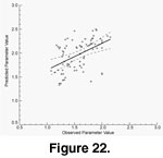
Figure 21 and Figure
22 show the quality of fit for Delaunay and TPS-interpolated data.
Once the link between climatic parameters and ecomorphologic parameters such as mean hypsodonty has been characterized, it is possible to use that relationship to interpolate a similar map for fossil data. Here we present an example for the large Tortonian mammals (the other Neogene continental stages have also been investigated in the same way).
Figure 20 shows the hypsodonty pattern for 100 Tortonian sites distributed throughout Europe. We plotted the results onto a palaeogeographic map drawn from
Rögl (1999) using palaeo-coordinates calculated from present-day coordinates, as well as stratigraphic and geographic positions.
Figure 21 and Figure
22 show the quality of fit for Delaunay and TPS-interpolated data. 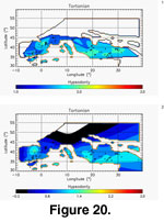 As for the present-day data, the bootstrap median of the median jackknifed mean interpolated values and its associated 95% confidence interval were independent of the size of the analyzed dataset. Here the low skewness of the hypsodonty distribution makes the two interpolation methods immune to very small-sized dataset bias. As already mentioned, the TPS method showed a wider bootstrapped 95% confidence interval than the Delaunay method due to its greater sensitivity to spatial heterogeneity. Indeed, the fact that the bootstrapped median jackknifed curves were uniformly shifted upwards for the TPS-interpolated Tortonian dataset indicates that this parameter is critical. Thus the TPS-interpolated values should be interpreted very cautiously.
 The Tortonian hypsodonty pattern broadly shows a North/South gradient with the highest values being mainly concentrated in the Iberian Peninsula and in the Greek-Iranian block
(Bonis et al.
1992). The central-eastern European localities (eastern France, Germany, Switzerland, Austria, and Romania) have lower mean values of tooth crown height. Note that the sharp decrease observed towards the northern boundary is an artefact of the interpolation method (an edge effect) due to a lack of data in high latitudes.
The Tortonian hypsodonty pattern broadly shows a North/South gradient with the highest values being mainly concentrated in the Iberian Peninsula and in the Greek-Iranian block
(Bonis et al.
1992). The central-eastern European localities (eastern France, Germany, Switzerland, Austria, and Romania) have lower mean values of tooth crown height. Note that the sharp decrease observed towards the northern boundary is an artefact of the interpolation method (an edge effect) due to a lack of data in high latitudes.
Here, IDL allowed us, through its interpolation methods and visualization facilities, to infer the species richness distribution and the tooth crown height biogeographic patterns of European large mammals. The present-day distribution of species richness produced by the IDL interpolation tool was consistent with previous works
(Baquero and Telleria
2001). Regarding ecomorphologic analyses, hypsodonty was largely related to two climatic parameters (precipitation and temperature) and closely followed a North/South climatic gradient, where the more arid and open environments were to the South.
 Based on these results, we computed the same ecomorphologic parameter for Tortonian large mammals localities and found out that the North/South broad gradient already existed by late Miocene time.
Our fossil map resolution suffers from the low number of localities (100) relative to the large geographic scale taken into account (the whole European continent), as well as from the absence of high latitudes localities due to glacial removal of Miocene continental sediments from northern Europe. Apart from these limitations and the previously discussed problem of spatial heterogeneity, the interpolation methods used in the Tortonian example, especially Delaunay triangulation, seem to produce reliable results.
