| |
BIOGEOGRAPHY AND GIS
Biogeography is concerned with locations of organisms in space. The fossil package implements a number of functions to assist in converting georeferenced datasets into formats useful for both graphing within R and exporting to GIS programs. R was originally created as a statistical language, but its ability to use and display geographic data is quite advanced for a non-GIS system. The sp package (Pebesma and Bivand 2005) along with a number of geographic libraries allows a user to put in data in a number of projections and change projection and datum. For a thorough treatment of spatial data analysis with R, I highly recommend
Bivand et al. (2008); here I provide only a cursory description of the topic.
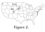 The simplest geographic function to use is likely create.lats(), which as mentioned previously can extract the locality data from a list of taxa occurrences. With the output from this function, a number of further analyses can be done. For example, it is often useful to have the distances between two points in space; this can be easily accomplished with the earth.dist() function, which returns a matrix of pairwise distances in kilometres (Figure 2). One note, however, is that the original matrix of locations must be in decimal degrees. Of course, the sp package provides functions to convert between coordinate systems if necessary. The simplest geographic function to use is likely create.lats(), which as mentioned previously can extract the locality data from a list of taxa occurrences. With the output from this function, a number of further analyses can be done. For example, it is often useful to have the distances between two points in space; this can be easily accomplished with the earth.dist() function, which returns a matrix of pairwise distances in kilometres (Figure 2). One note, however, is that the original matrix of locations must be in decimal degrees. Of course, the sp package provides functions to convert between coordinate systems if necessary.
 Biogeography is concerned with species locations in space, and the sampling distributions of those species can cause some interesting effects in diversity calculations, namely the well researched species/area effect (Arrhenius 1921;
Gleason 1922;
Preston 1960;
Connor and McCoy 1979;
Rosenzweig 1995). Although palaeontology often pays little attention to this effect,
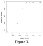
Carrasco et al. (2005) have shown that it does hold true in fossil data sets. As a way to observe these effects efficiently, I have created the function sac() that can create a summary species area curve for a data set (Figure 3). As its arguments, it takes a table of longitude/latitude and a species occurrence matrix. It makes use of another function called earth.poly(), which can take a table of locations and calculate which points create the vertices for a minimum spanning polygon/convex hull, as well as calculate the true geographic area of the polygon. Biogeography is concerned with species locations in space, and the sampling distributions of those species can cause some interesting effects in diversity calculations, namely the well researched species/area effect (Arrhenius 1921;
Gleason 1922;
Preston 1960;
Connor and McCoy 1979;
Rosenzweig 1995). Although palaeontology often pays little attention to this effect,
Carrasco et al. (2005) have shown that it does hold true in fossil data sets. As a way to observe these effects efficiently, I have created the function sac() that can create a summary species area curve for a data set (Figure 3). As its arguments, it takes a table of longitude/latitude and a species occurrence matrix. It makes use of another function called earth.poly(), which can take a table of locations and calculate which points create the vertices for a minimum spanning polygon/convex hull, as well as calculate the true geographic area of the polygon.
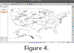 Though the R environment is powerful when analysing GIS data, it lacks a large amount of visual interactivity with the data. Often, it is simply easier to use a GIS program to view geographic data, and as such I have tried to make it as simple as possible to move geographic data out of R. Currently the package provides helper functions for exporting both geographic points (lats2Shape()) and MSTs/MSNs (msn2Shape) to shapefile format using the package shapefiles (Stabler 2006). To use the functions, you need the shapefile package available on your system; the package can be downloaded using the install.packages(shapefiles) command. Once the shapefiles have been created, they can be saved using the write.shapefile() command. The shapefiles can then be loaded in any GIS program (Figure 4). Though the R environment is powerful when analysing GIS data, it lacks a large amount of visual interactivity with the data. Often, it is simply easier to use a GIS program to view geographic data, and as such I have tried to make it as simple as possible to move geographic data out of R. Currently the package provides helper functions for exporting both geographic points (lats2Shape()) and MSTs/MSNs (msn2Shape) to shapefile format using the package shapefiles (Stabler 2006). To use the functions, you need the shapefile package available on your system; the package can be downloaded using the install.packages(shapefiles) command. Once the shapefiles have been created, they can be saved using the write.shapefile() command. The shapefiles can then be loaded in any GIS program (Figure 4).
>data(fdata.lats)
>shape.lats<-lats2Shape(fdata.lats)
>fdata.dist<-dino.dist(fdata.mat)
>fdata.mst<-dino.mst(fdata.dist)
>shape.mst<-msn2Shape(fdata.mst,fdata.lats)
|