|
|
|
Correlations and Base SetAs explained in the introduction, the selection of a proper base set is crucial in the analysis of correlations. In selecting the base set it is important to understand for what purpose the correlations are used: we use the correlations as indicators of some effects between pairs of species. The selection of the base set can be used to choose the effects for which we want to test. The situation is analogous to the design of controlled experiments. We would like to design an experiment such that only the variables that we are interested in affect the results. For example, if we would like to rule out the effects of large scale geography we would choose the locations so that we can compare only nearby sites. In analyzing ecological data we usually have the data given and cannot choose how the experiment is designed (for example, where and when the find sites are located). Lacking the ability to design the experiment we use base set selection to control the variables of whose effects we want to study. The price we pay is the reduction of power: with a proper selection of the base set we can (as explained below) control to some degree the variables that we want to study, but the more we restrict the base set the less locations it will include and the statistical test will be correspondingly less powerful. For example, consider global presence-absence data where we have a set of present-day locations. Assume that we study the correlation between two species that occur only within Africa. 1. We can take all locations in the base set. We are likely to obtain a significant positive correlation, because in most of the locations (all locations outside Africa) neither of the species occur. The correlation is real, but the reason for it is trivial: the species are clearly not independently distributed, because both of them occur only in Africa, and therefore they are correlated. 2. We can use all African locations as a base set. If we choose some pre-defined set of locations (such as Africa) as a base set we can exclude the effect of this set of locations to the correlation. In this case, if we use Africa as a base set, and if we still observe a statistically significant correlation, we know that the correlation must be due to some other reason than both of the species occurring only in Africa. In other words, we have controlled the experiment so that the effect of Africa does not affect the results. In many applications, a more reasonable choice than a continent could be, e.g., the area covered by a given biome. As a result, if we would observe a correlation, it would be due to some other reason than the biome only. 3. We can use the union of the areas of occurrence of the species as a base set. Often, there may be no straightforward pre-defined area (such as Africa or a given biome) that we could use as a base set. If this is the case, one can use the locations within the union of the areas of occurrence of the two species as a base set. This choice guarantees that any observed correlation is due to some effect that takes place within the area of occurrence of the two species. Notice that this choice is closest in spirit to the Jaccard and like indices, which ignore the locations in which neither of the species occur. As discussed before, Jaccard and like indices are however not proper indicators for correlation: they can give high co-occurrence counts even when there is no correlation, like in the example of Table 2. 4. We can use the intersection of the areas of occurrence as a base set. If we want to rule out the effect of the large-scale areas of occurrences altogether, then we can use as a base set the locations within the intersection of the areas of the occurrences of the two species. If we observe a correlation it must be due to a reason not related to the areas of occurrences. In this paper, we use the smallest rectangle that can be used to enclose all occurrences of a species as an area of occurrence. The union or intersection of these areas is then used to define the base set of locations. Rectangles are not rotationally invariant, which means that their definition is dependent on the direction of the coordinate axes. For improved precision, smallest rectangles can be replaced with more advanced structures, such as convex hulls, i.e., minimal polygons containing all the locations where the species occurs. The fossil data consist of locations that have a specific age in addition to the spatial location. We can define the lifetime of the species as the time interval between and including the earliest and the latest occurrence of the species. If we take all locations from all times into account the results are easily dominated by the trivial fact that the lifetimes differ for most pairs of species. Typically, we want to exclude the effect of time from the analysis. Therefore, we can use as a base set the locations within the intersection of the lifetimes of the respective species. It follows that if we observe any correlation, it must be due to some reason that is not related to the lifetimes of the species. To demonstrate the effect of different base set selection criteria, we present synthetic data for two African species A and B. Using different geographic selection criterias, we calculate Fisher's Exact Test, mid-P, and as an example of a typical association similarity index, the Jaccard index. For statistical significance we use the level 0.05, without multiple hypothesis testing correction.
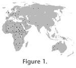
We look into this negative correlation more closely. Figure 1 shows areas of both species as dashed rectangles. The base set can be selected from these areas by either looking at them both, i.e., the union of areas, or by looking only into the intersection of the two areas, i.e., where we have evidence for both of species occurring. Table 5 shows occurrence counts in the case of union of areas. Looking at Table 5, we see significant negative correlation as can be read from the very low p-value. It could be argued that the two species are dissimilar, maybe suggesting an interaction that would not allow the two species to co-exist. However, when looking at the base set of intersecting areas, as reported in Table 6, we cannot see significant correlation. Table 6 is most suited for analysing interactions between species, and it does not support hypothesis of dissimilarity, possibly due to lack of data. Dissimilarity in Table 5 could be explained by geography, as the two species have different areas of occurrence. In the area where both species occur there is no strong evidence of interaction as seen from Table 6. What we see in the example above is fundamentally related to spatial autocorrelation: the probability of occurrence and co-occurrence of the species depends on the geographic locations of the occurrences. Fisher's Exact Test does not account for spatial autocorrelation directly. Instead, our approach is to use base set selection to control the spatial effects. By making this choice explicit we do not hide uncertainties related to spatial autocorrelation and make the analysis process easier to understand and evaluate. In the example case, we examined how accounting for spatial effects changed the results significantly. Summarizing the above discussion, before we can choose a base set, we have to decide which effects we want to study. The answer (whether there is a correlation or not) depends on which types of effects we want to study. Naïve selection of a base set leads to trivial results. For example, if we select all locations as a base set then any observed correlation may be simply due to different areas of occurrences and differences in the lifetimes of the species. Typically we are not interested in these variables because they are trivial to notice and understand even without any correlation analysis. Therefore, we need to bound the base set such that the effect of known or uninteresting variables is eliminated. |
|