 Idealized landmark-based geometric reconstructionsof poorly preserved fossil material:
A case study of an early tetrapod vertebra
Article number: 15.1.2T
https://doi.org/10.26879/274
Copyright Palaeontological Association, February 2012
Author biographies
Plain-language and foreign language summaries
PDF version
Submission: 16 March 2011. Acceptance: 22 November 2011
{flike id=165}
ABSTRACT
Three-dimensional (3D) digital models of bone morphology are used frequently in paleontology and anthropology. Because fossils are often fragmentary or distorted, it often becomes necessary, for either aesthetic or practical reasons, to create an idealized version of digital skeletons. We propose a method for building landmark-based geometric reconstructions of fossil bones in 3D graphics software using CT or laser scan data as a template. This method does not require specialized software or artistic expertise. It allows control of local mesh density, specification of important landmarks and major planes, elimination of large holes and extraneous structures, and interactive adjustment of 3D shape by moving a small number of vertices to correct minor taphonomic deformation. The result is a simple, illustrative, and accurate model that can be used for diverse analytical and visualization applications, including reconstructions of incomplete fossils, watertight models for mass and center of mass approximation, base meshes for thin plate spline warping, and intermediates in an incomplete series via "morphing." To demonstrate the method, we applied it to reconstruct a dorsal vertebra from the basal tetrapod Acanthostega gunnari. We validated our methodology with linear and geometric morphometric comparisons of our reconstructions both against the original scan data and between three different operators. Based upon four linear measurements, the average deviation of the models from the original was minimal, showing that the method preserves the proportions of the original fossil. We found no statistically significant shape difference between models built by different operators, demonstrating that the method is repeatable.
Julia L. Molnar. Department of Veterinary Basic Sciences and Structure and Motion Laboratory, The Royal Veterinary College, AL97TA, United Kingdom. jmolnar@rvc.ac.uk
Stephanie E. Pierce. University Museum of Zoology, Department of Zoology, University of Cambridge, Cambridge, CB2 3EL, United Kingdom and Department of Veterinary Basic Sciences and Structure and Motion Laboratory, The Royal Veterinary College, AL97TA, United Kingdom. spierce@rvc.ac.uk
Jennifer A. Clack. Department of Zoology, University of Cambridge, Cambridge, CB2 3EL, United Kingdom. j.a.clack@zoo.cam.ac.uk
John R. Hutchinson. Department of Veterinary Basic Sciences and Structure and Motion Laboratory, The Royal Veterinary College, AL97TA, United Kingdom. jrhutch@rvc.ac.uk
KEYWORDS: Acanthostega; idealized model; digital skeleton; fossil reconstruction; NURBS modeling; visualization
FINAL CITATION: Molnar, Julia L., Pierce, Stephanie E., Clack, Jennifer A., and Hutchinson, John R.. 2012. Idealized landmark-based geometric reconstructions of poorly preserved fossil material: A case study of an early tetrapod vertebra. Palaeontologia Electronica Vol. 15, Issue 1; 32,18p;
palaeo-electronica.org/content/issue-1-2012-technical-articles/165-digital-fossil-restoration
INTRODUCTION
Background
Three-dimensional digital models of bone morphology derived from laser surface scans, computed tomography (CT), or mechanical digitizing are used frequently in paleontology and anthropology. Virtual fossils can be manipulated using computer programs in order to, for example, correct taphonomic distortion, study basic anatomy for its own sake or for phylogenetic analysis, examine differences in bone shape between individuals or species using morphometrics, analyze biomechanical parameters, and produce interesting and informative scientific visualizations (reviewed in Bookstein, 1997a; Zollikofer et al., 1998; Lewin, 2002; Alexander, 2006; Sutton, 2008; Gunz et al., 2009).
In fossil reconstruction, digital models permit manipulations that would be impossible with specimens or casts, such as "digital dissection" of inaccessible areas without risking damage to the specimen, mirroring forms and combining parts of different specimens, virtually articulating structures that are too massive to move in reality or embedded in matrix, and visualizing internal structures using transparency and virtual endocasts (e.g.,Witmer et al., 2008;Zollikofer and Ponce de León, 2005). For example, Zollikofer et al. (2005) used digital retrodeformation to restore the skull of Sahelanthropus tchadensis and help diagnose it as a fossil hominid rather than an ape.
In the field of biomechanics, digital skeletons of extinct animals increasingly are being used in novel ways, including estimating joint range of motion and posture (e.g., Stevens and Parrish, 1999; Mallison, 2010b, c), as a framework for soft-tissue reconstructions to estimate mass parameters (e.g., Henderson, 1999; Motani, 2001; Hutchinson et al., 2007; Bates et al., 2009, 2010; Mallison, 2010a), and in simulation software to derive muscle moment arms and energetic costs of locomotion (e.g., Hutchinson et al., 2005; Nagano et al., 2005; Sellers and Manning, 2007; Sellers et al., 2009, 2010; Bates et al., 2010). Digital skeletons also can be used to calculate bone stresses and strains using finite element analysis (FEA) (e.g., Rayfield et al., 2001; Moreno et al., 2007; Snively and Russell, 2002; Strait et al., 2009; Wroe et al., 2010). Finally, digital models are invaluable in the arena of visualization to accompany photographs in manuscripts and web sites, plan or augment physical displays in museums (and even create physical models through rapid prototyping), and share data between researchers in different parts of the world (Mallison et al., 2009).
For some of these applications, and especially when using virtual skeletons for visualization, it often becomes necessary to create an idealized version of fossil morphology. This requirement can arise when using computer software designed to work with medical imaging data (such as some biomechanics software) that requires continuous, closed surface geometry, for visualization applications when smoothness and low computational cost are desirable, or for facilitating correction of distortion (Stevens, 2002; Hutchinson et al., 2005; Sellers et al., 2009). While generally readily available for extant species, high quality scan data are less available for extinct animals because fossils often are incomplete or broken and may show up poorly on CT scans. Large and/or mounted specimens that are unsuitable for CT scanning may be captured using a laser surface scanner or a mechanical digitizer, but this method often yields meshes with large gaps where the scanner beam cannot reach, imperfectly aligned surfaces, and extraneous elements such as mounting rods.
With these challenges in mind, we propose a method to build idealized geometric models in 3D graphics software from which biomechanical, volumetric, morphometric, and other data can be extracted in the absence of a well-preserved, complete specimen or comprehensive scan data. Our goal was to find a happy medium between using collections of geometric primitives (such as cubes and cylinders) as proxies for bones and the more time consuming and computationally intensive approaches that are the standard in paleoanthropology (see below), some of which are not applicable to specimens with unique morphologies. Here we use the triangulated mesh derived from a CT or laser scan as a template to model a landmark-based geometric reconstruction of a tetrapod vertebra. Our method is reasonably simple and repeatable because the placement of vertices is dictated by the location of biological and geometric landmarks and constrained to the surface of the template mesh. We borrow from computer graphics techniques by planning the model's geometry around biologically meaningful structures such as body axes and articulations.
Related Work - 3D Virtual Fossil Reconstruction
Driven by the challenges inherent in working with fossils, very sophisticated methods of fossil reconstruction have been developed over the years. Modern computer-based 3D methods using CT and laser scan data fall into two general categories. The first is "jigsaw puzzle" reconstruction and/or hole-filling to correct brittle deformation (e.g., Ponce de León and Zollikofer, 1999; Zollikofer et al., 2005). The second is warping to correct plastic deformation using bilateral symmetry or knowledge of the direction of deformation (e.g., Bookstein, 1989; Hamada et al., 1991; Motani, 1997; Ponce de León and Zollikofer, 1999; Ogihara et al., 2006; Angielczyk and Sheets, 2007; Gunz et al., 2009). In the more difficult cases, researchers may attempt to extrapolate missing morphological information based upon homology ("statistical reconstruction"; Gunz et al., 2009) or geometry ("geometric reconstruction"; Zollikofer and Ponce de León, 2005). Extrapolation is useful for such tasks as estimating the volume of non-watertight "leaky" structures and visualizing specimens for display or comparison. While data derived from extrapolation are not guaranteed to be accurate, one can obtain a good estimate of the range of possible values by repeating the process using different methods and assumptions (Zollikofer and Ponce de León, 2005). Of course, one always must be explicit about the methods used and which data have been extrapolated. Geometry- and homology-based extrapolation methods both have strengths and weaknesses and are appropriate in different scenarios (Zollikofer and Ponce de León, 2005).
Homology-based extrapolation takes advantage of biologically homologous landmarks to compare a complete reference specimen with the incomplete target specimen. A thin-plate spline (TPS) function based upon the difference between landmark configurations of the reference and target specimens defines a "deformation space." The vectors from the deformation space are then used to warp the reference specimen to match the landmark configuration of the target (Bookstein, 1997b). Although this approach yields highly detailed, realistic-looking results, it is important to realize that it is primarily a visualization tool (Bookstein, 1997a). The TPS function interpolates deformations geometrically between landmark points, and therefore it does not confer definite biological information beyond (or between) the landmark data. Because of this, it is important to choose a reference specimen that represents the plesiomorphic condition to avoid biasing the results towards the derived morphology of the reference specimen (Gunz et al., 2009). To avoid this problem, some researchers have used statistical or geometric morphometrics to analyze multiple related species and produce a "consensus" landmark configuration (Wiley et al., 2005). Others have relied on an idealized, artist-generated template (Allen et al., 2003; Souter et. al, 2010).
Regardless of the method of template generation employed, homology-based extrapolation requires one or more complete specimens, which share a set of biologically homologous landmarks with the target specimen (Mitteroeker and Gunz, 2009). However, it is rare in paleontology to have a large number of complete specimens within a species. Geometry-based extrapolation circumvents the problem of reference specimens by relying instead upon the preserved geometry of the original specimen. A deformable template with the desired topology, often a spline surface, is created and then warped using the energy-minimum principle to match the specimen's configuration with minimum internal energy (conceptually similar to shrink-wrapping) (Zollikofer and Ponce de León, 2005). With respect to re-creating the original anatomy, this approach is probably less accurate than homology-based extrapolation; however, it avoids species bias and is a considerably simpler operation.
 Rather than using splines to alter polygonal geometry, other researchers build spline contours from their data in the initial acquisition phase by using mechanical digitizing rather than CT or laser scanning (e.g., Hutchinson et al., 2005, 2007; Mallison et al., 2009). In this procedure, a series of contour lines are marked upon the physical specimen and the digitizing apparatus is moved along the bone's surface, collecting 3D spatial coordinate points. The points are connected with splines to make contour lines, and the contour lines are lofted to create a non-uniform rational B-spline (NURBS) surface. Alternatively, digitized points can be saved as a point cloud, and a NURBS surface can be generated automatically using 3D software such as Rhinoceros (www.Rhino3d.com) or Geomagic (www.Geomagic.com). The advantages of mechanical digitizing over laser and CT scanning are cost and file size; additionally, it works well for fossils that are too large for CT scanning, and it can make reconstruction simpler due to the properties of NURBS surfaces (Mallison et al., 2009).
Our method of landmark-based geometric modeling addresses some of the problems of fossil reconstruction by combining elements of several approaches. Like Ponce de León and Zollikofer (1999) and others, we use a 3D surface derived from a CT scan of a specimen to place geometric and biological landmarks (Figure 1), and like Allen et al. (2003) and Souter et al. (2010), we construct our model using computer graphics-inspired techniques to maximize accuracy of shape while minimizing vertices. Similar to geometric extrapolation, we use a type of spline function to interpolate between landmark points without reference to a homologous specimen, and similar to mechanical digitizing, we extract a subset of surface points to build a simplified, idealized 3D representation of the specimen using NURBS curves.
Polygonal Surfaces, Splines, NURBS, and Landmarks
A major component of our reconstruction method is the conversion of bone geometry from a polygonal surface (stereolithography or STL file format) to a spline surface using geometric landmarks. Commonly used to represent 3D digital surfaces including CT and laser scan data, STL files consist of a set of contiguous faces, each usually defined by three vertices and a normal vector that differentiates between the inner and outer surface. Polygonal surfaces such as STLs are discontinuous; that is, their tangents change sharply at each edge. While STL files are useful because they are relatively easy to extract from 2D slices (CT scans) and point clouds (laser scans and mechanical digitizers) and are widely supported by modeling and analysis programs, sometimes it is desirable to construct models using continuous (spline) surfaces. Splines are useful in modeling organic shapes because they smoothly interpolate between points, requiring fewer control vertices to describe curving surfaces. In the biological sciences, spline surfaces are commonly used in paleontology to construct deformable templates (e.g., Zollikofer and Ponce de Leon, 2005) in geometric morphometrics to describe shape variation (Bookstein, 1989) and visualize extreme morphologies (e.g., Pierce et al., 2008; Pierce et al., 2009), and in FEA to transform existing FE models to match new morphologies (e.g., Stayton, 2009).
Splines are curves or surfaces defined mathematically by piecewise polynomial functions. They interpolate between operator-defined points or "knots" to describe a curve that minimizes bending energy between knots (Bookstein, 1989). NURBS are a category of splines used in scientific visualization, industrial design, and, less frequently, paleontology. For example, Strait et al. (2009) constructed a solid structure of a skull belonging to Australopithecus africanus using NURBS in a 3D modeling program for the purpose of finite element analysis (FEA), and NURBS surfaces have been used, for example, to reconstruct idealized skeletal elements for biomechanical analysis of Tyrannosaurus rex (Hutchinson et al., 2005) and to approximate soft tissue volume in order to estimate center of mass for T. rex and the sauropodomorph dinosaur Plateosaurus engelhardti (Hutchinson et al., 2007; Mallison, 2010a).
Geometrically, "landmarks" or "landmark points" are local extrema that correspond between objects. "Biologically homologous landmarks" are a subset of landmark points for which "objectively meaningful and reproducible counterparts" exist between all forms (Bookstein, 1989). Not all landmarks are biologically homologous, and it is necessary to use only biologically homologous landmarks when comparing specimens of different species. However, when simply comparing between shapes, any identifiable geometric landmarks can be used. In this paper, the unqualified term "landmarks" refers to geometric landmarks.
MATERIALS AND METHODS
Purpose of Study
 To demonstrate the method of landmark-based geometric reconstruction, we applied it to reconstruct a dorsal vertebra (neural arch, intercentrum, and pleurocentra) from the basal tetrapod Acanthostega gunnari, a Devonian tetrapod with a morphology intermediate between aquatic lobe-finned fishes and fully terrestrial early tetrapods. Acanthostega is widely considered to be a critical sister taxon of modern terrestrial vertebrates (Ahlberg and Milner, 1994; Coates, 1996; Clack, 2002; Coates et al., 2002; Carroll, 2009). The locomotor behavior of Acanthostega is therefore of utmost interest to evolutionary biologists for reconstructing the evolution of terrestrial locomotion in Tetrapoda (currently under study by the authors). However, fossils of the animal are scarce, and those available have low matrix-bone contrast, making them difficult to translate into high-fidelity 3D models. We validated our methodology with geometric morphometric comparisons of our reconstructions both against the original mesh derived from CT scan data to test their accuracy and between operators to evaluate repeatability.
CT Datasets
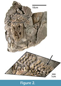
A portion of the Acanthostega specimen containing neural arches, intercentra, and pleurocentra (Geological Museum, University of Copenhagen: MGUH f.n. 1227; Figure 2) was micro-CT scanned with a Metris X-Tek HMX ST 225 CT scanner (slice increment: 0.169, pixel size: 0.085 mm).
Segmentation of CT data
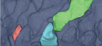
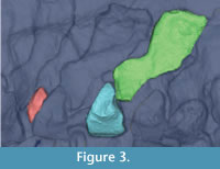 The CT dataset was imported into Mimics (Materialise Inc.); Leeuwen, Belgium), a commercial image processing program for segmenting CT and MRI data and constructing triangulated 3D surface meshes. Because it did not contain sufficient contrast for automatic segmentation, the Acanthostega dataset was processed by hand: on each CT slice, the area representing an individual bone was selected using the Lasso tool and added to a mask (Mimics image). The choice of vertebra was dictated by preservation: we exported the most complete and apparently least distorted vertebra, thought to be the 21st dorsal.Acanthostega has multipartite vertebrae, each consisting of a neural spine, intercentrum, and paired pleurocentra (Coates, 1996). Only the left half of the vertebra is preserved in this specimen, and the medial surface is not distinguishable. The pleurocentra were not preserved for the 21st dorsal vertebra and were segmented from a different vertebra in the same series (19th dorsal). Each element was volume-rendered using the "Medium" setting (Figure 3), and its surface was exported as a separate STL file. A smoothing filter (Laplacian smooth, 1 iteration) was applied in the free mesh processing software MeshLab to simplify visualization. Because of the large number of vertices in the STL file (over 130,000), this operation had a negligible effect upon the geometry.
Creating NURBS Models in Autodesk Maya
STL files were imported into Autodesk Maya, a 3D animation and modeling program for computer graphics (Autodesk Inc.; trial version free to download). When building an idealized model of a bilaterally symmetrical form, such as a vertebra, it is generally preferable to reconstruct only one half and then join it with its mirror image, as was done in this case. Had both halves of the vertebra been preserved, we would have divided the mesh along its mid-sagittal plane and removed one half before proceeding (see Appendix for procedures in Maya).
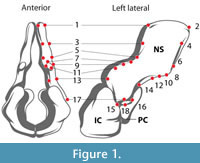
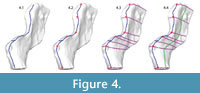 Mapping landmarks onto the 3D surface. A UV map was created for the mesh to allow "painting" on its surface with the 3D Paint tool. Contours delineating major planes were marked in blue (anterior, posterior, lateral, and medial; the superior edge of the neural spine and the diapophysis [rib articulation] of the transverse process are modeled separately). Major biological and geometric landmarks, located at the intersections of major planes and the boundaries of important biological structures, were marked in red. Perpendicular contour lines were added (violet) connecting corresponding landmarks on opposite edges of the planes (e.g., the anterior superior tip of neural spine was connected to the posterior superior tip of neural spine). Subsidiary contours were added (green) roughly parallel to the plane contours to define the medial and lateral surfaces. The number of subsidiary contour lines is a matter of judgment; each additional contour that is added will increase both the complexity and the fidelity of the model. The result was a generally evenly spaced grid that became more closely spaced in areas of special interest and/or geometric complexity (Figure 4).
Creating contour curves and NURBS surfaces. NURBS terminology in Maya is similar to that used in the introduction ("Polygonal surfaces, splines, NURBS, and landmarks"). When creating a curve in Maya, knots are referred to as "Edit points" and the segment between points as a "span." "Degree setting" refers to the degree of the polynomials that describe a curve or surface.
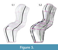
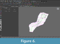
The mesh was made "Live" in order to constrain the knots of the NURBS curves to the mesh surface. This step ensured that the points used to create the contours would exactly correspond to data points on the template mesh. NURBS curves were created following the blue lines (major plane junctions) and green lines (medial and lateral surfaces) with an edit point at each intersection with the purple lines (perpendicular contours) (Figure 5, Figure 6).
 |
 |
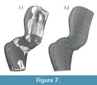
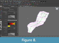
The curves were "lofted," or joined by interpolated NURBS surfaces, to create a continuous NURBS shape (Figure 7, Figure 8). The purpose of the painted grid was to create a set of curves that was optimal for lofting. It ensured that each curve was created using similarly spaced knots and the same number of spans, improving the appearance of the NURBS surface. Additionally, since curves were created following a set of fairly evenly spaced, non-intersecting lines, it was easy for the program to create a smooth surface in the perpendicular direction.
 |
 |
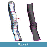
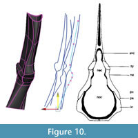
Adjustments and extrapolation of missing surfaces. This point in the reconstruction process is the ideal one to adjust the model to better fit the data or to correct deformation. This is because the NURBS surface is controlled by the NURBS curves and is updated dynamically as their shapes are changed. The NURBS surface was selected and moved to one side so that the curves could be selected more easily. Then, using the surface to visualize the results, the curves were adjusted by moving the knots. First, areas on the model that did not match the template mesh well were identified and improved by sliding knots along the surface of the template mesh (Figure 9). Next, knots were adjusted by eye (without snapping to the template mesh) to correct presumed scanning errors and taphonomic deformation. In this case, the medial surface of the intercentrum and pleurocentrum, not distinguishable from the scan, were altered to match Coates' (1996) two-dimensional reconstruction (Figure 10).
 |
 |
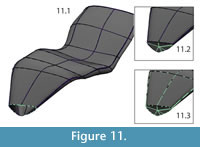
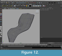
Closing open edges. After all adjustments had been made, the open ends of the surfaces were either closed with facets (e.g., the diapophysis on the transverse process of the neural arch) or left open to be joined with bilaterally symmetrical halves after mirroring (e.g., the inferior edge of the left half of the intercentrum) (Figure 11, Figure 12).
 |
 |
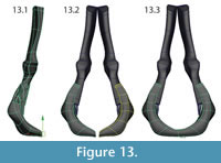
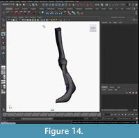
Mirroring and attaching. After all elements had been modeled, they were grouped and mirrored. The two halves of the intercentrum were attached at the mid-line (Figure 13, Figure 14).
 |
 |
Alternative Techniques
Creating polygonal models. This model building technique also can be easily adapted to create polygonal models. To do so, change the options when creating contour curves from "3 Cubic" to "Linear" and the output geometry from "NURBS" to "Polygons." Although polygonal models are not as smooth as NURBS models, they are more flexible with regards to modifying shape and they can be exported as .OBJ files without conversion.
Automating knot insertion for complex models. Optionally, it may be useful to partially automate knot insertion when creating surfaces that are more complex than our examples. To do this, simply create curves as described above and then automatically insert additional knots within each span. The new knots will not necessarily lie upon the template surface, but they can be "snapped" to the surface as in Figure 9. Although it requires an extra step, this technique makes it easier to ensure that multiple complicated curves have the same number of spans distributed with the same density along their lengths.
Validation and Repeatability
To evaluate accuracy and repeatability, the procedure was performed a total of 15 times upon a neural arch of Acanthostega by three different operators (JLM, JRH, SEP). JLM had been trained to use Maya, while JRH and SEP had never used the program before. The two untrained operators were instructed in the use of the Maya interface by JLM and then given a file with the template mesh and a printout of the instructions contained in the Materials and Methods section. Each operator performed the model building procedures five times independently. All completed models were converted to polygons (Modify>Convert>NURBS to Polygons>Options; Type: "Quads," Tessellation method: "Standard fit") and exported as .OBJ files. The .OBJ files were converted to .PLY files in MeshLab. The original .STL file that had been used as a template also was converted into a .PLY file in MeshLab. All .PLY files were imported as surfaces into the program Landmark (version 3.6; free to download from EvoMorph).
 Linear morphometrics. To determine whether the dimensions of the original specimen had been preserved in the models, four linear measurements from each surface were taken and analyzed. Six 3D landmark points were placed at corresponding locations on each model and on the original specimen: anterior and posterior tip of neural spine, anterior and posterior edge of neural arch at base of neural spine, and anterior and posterior tip of diapophysis. These points were chosen because they were easiest to identify consistently on each surface. Distances between the landmark points were used to extract four linear measurements: neural spine width at tip (D1), neural spine width at base (D2), transverse process width at tip (D3), and total neural arch height (D4) (Figure 15).
Shape analysis. In order to capture shape information in addition to dimensions, additional 3D landmark points were semi-automatically placed in Landmark on the surfaces of the original scan data and the 15 idealized models. First, the six points on each surface that had been used in the previous step to take linear dimensions were identified as corresponding landmarks between surfaces. Next, six patches of landmark points were placed on the surface of the original specimen: two on the neural spine (one on the medial aspect and one on the lateral), two on the arch between the zygapophyses, and two on the transverse process. Each patch consisted of nine landmarks and 16 semilandmarks. The use of patches allowed placement of multiple landmark and semilandmark points at one time, and it also facilitated the establishment of correspondence between landmarks on different models. The patches were semi-automatically applied to the remaining surfaces using the original mesh as the reference ("atlas") surface as described in the Landmark documentation (Figure 15). The six patches were identified as corresponding sets of landmarks. Finally, a total of 66 landmarks and 96 semilandmarks were exported from each model. Landmark coordinates for all models were superimposed using the Generalized Procrustes Method to remove the effects of position, orientation and scale from the data set. To assess and visualize shape variation, the aligned data were then converted into shape variables (i.e., partial warp and uniform component scores) and subjected to a principal components analysis (PCA) in the geometric morphometrics toolkit Morphologika (O'Higgins and Jones, 2006).
Data analysis. Variation in linear measurements between the idealized models and the original specimen was visualized using a box and whisker plot. Because there was only one original specimen, calculation of statistical differences between the idealized models and the original were not possible; we could only look at inter-operator repeatability. To analyze shape variation between models built by different operators, a MANOVA was performed using principal component (PC) scores that accounted for 5% or more of the variation. Exploratory and statistical analyses were performed in the paleontological statistics software package PAST (version 2.07).
RESULTS
Idealized Model
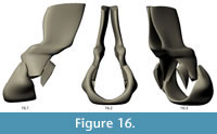
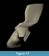
The final NURBS model of the complete dorsal vertebra of Acanthostega is shown in Figure 16 and Figure 17. The model has 210 knots including contour lines and facets, and it represents our best estimate of the original 3D morphology of the bone based on available information.
 |
 |
 Validation and Repeatability
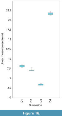
Linear measurements. The average difference in the linear measurements between the models and the original mesh was 2.0-6.1% (<0.5 mm in all dimensions) (Table 1). By percentage, the greatest difference between the models and the original specimen was transverse process width at tip (6.09% or 0.22 mm), and the smallest difference was in total neural arch height (2.00% or 0.44 mm). The likely reason that transverse process width was the least accurate is that the tip of the transverse process was difficult to model because the 'knots' were very close together. Between all models (not including the original specimen), the standard deviation of linear measurements was 0.21-0.34 mm (Figure 18).
Shape variation. The Generalized Procrustes superimposition displays little variation in landmark positioning (Figure 19). The PCA shows that groups of models created by the experienced operator (green diamonds) overlap with those created by both of the inexperienced operators (blue squares and pink circles), which also overlap with each other (Figure 20). 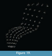 However, the groups of idealized models do not overlap with the original specimen, indicating a departure from the original shape, an effect probably due to the models' smoother surfaces. Nonetheless, visualization of extreme morphologies along PC1 and PC2 shows little variation between landmark configurations (Figure 20). PC1, which accounts for 24.3% of the variation, appears to represent slight anterior-posterior changes in the length of the neural spine and the sharpness of the transition between the body of the neural arch and the transverse process. PC2, which accounts for 14.4% of the variation, appears to represent slight changes in the width of the narrowest portion of the neural arch (Figure 20).
 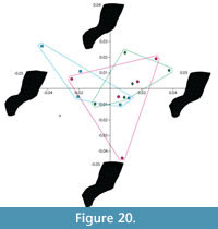 A MANOVA of the principal components that accounted for >5% of the variation (PCs 1-7) showed no significant difference in shape between models created by different operators (Pillai trace F value =1.357, p-value: 0.228) supporting the repeatability of the methodology.
DISCUSSION
Rationale
We chose this approach to the problem of working with incomplete and low-quality fossil data in order to maximize simplicity of execution and minimize the propagation of noise while preserving gross morphometric measurements and realistic anatomy. Alternatively, we could have attempted to retrodeform the element by using a TPS function to warp the mesh vertices and reconstruct missing portions using a deformable template (e.g., Zollikofer and Ponce de León, 2005). Similarly, if a complete specimen with sufficient homologous landmarks were available, we probably could have achieved good results using a TPS interpolation function to warp the template specimen (e.g., Zollikofer et al., 1998). However, because the vertebrae of Acanthostega are morphologically distinct from those of its closest known relatives, and because we needed only a form consistent with the preserved bone geometry and not a detailed surface, it was more appropriate in this case to use generic modeling software to create an idealized version that was structurally simple enough to retrodeform by adjusting vertices directly. On the other extreme, we could have built a less realistic model from simple shape primitives based on measurements taken from the fossils (e.g., Stevens, 2002; Souter et al., 2010). In this case a more realistic approach was judged preferable both for visualization purposes and to allow us to incorporate the maximum amount of available data into our model.
Advantages
The advantages of our landmark-based geometric modeling method are flexibility, control, and simplicity. There are no requirements for the input data in terms of file size or mesh quality, although better scans produce more accurate models. By drawing contours using landmark points placed directly on the surface of the mesh, the operator can control local mesh density and define major planes, adapting the approach to fit the morphology of a particular specimen and the desired parameters of the model. Multiple meshes can be integrated, large holes filled, and extraneous structures ignored, yielding an idealized form. However, because the model is constructed using the original specimen as a template, its creation does not require artistic expertise, and its dimensions will closely match the original. Operators who had never used the program before were trained in the Maya interface and completed their first simple model (neural spine of Acanthostega) in approximately 1 hour (subsequent models took 15-30 minutes). We found no statistically significant shape difference between models created by different operators, whether or not they were experienced in using 3D modeling software. In short, this is a reliable and repeatable method for building idealized versions of poorly preserved fossil material.
Surfaces generated from laser or CT scanners typically require extensive processing to reduce file size, close holes, and correct errors in automatic surface generation. Using our method, processing and reconstruction can be combined into one step. In our example, a mesh with 134,369 vertices (the neural arch of Acanthostega) was converted to a NURBS surface with only 44 control points. This reconstruction method allows the operator to specify important landmarks and major planes and interactively to adjust the shape of surfaces between them, as opposed to decimation and re-meshing (e.g., Schroeder et al., 1992; Alliez et al., 2005), which automatically decreases vertex counts using a density function. Finally, because it is constructed from NURBS surfaces, the shape of the model can be adjusted easily and interactively to correct minor taphonomic deformation by moving a small number of vertices (e.g., Hutchinson et al., 2005). The result is a simple, illustrative, and substantially accurate model that can be used for diverse analytical and visualization applications.
Limitations
Despite its advantages in terms of flexibility, the lack of automation in our approach imposes several important limitations. Although we have tried to standardize the process as much as possible, each subsequent model extrapolated from a single specimen will be slightly different. This effect may be compounded when models are created by different operators. However, we investigated the repeatability of model creation by three different operators with a predetermined set of landmarks and plan for the mesh structure and found no significant difference between the shapes created by different operators. Although there were shape differences between the model and the original specimen, likely due to smoothing of the surface, the average deviation in terms of linear morphometrics was minimal. For the purpose of biomechanical analysis, preserving linear dimensions is particularly important because they affect such biomechanical indices as cross sectional area and lengths of lever arms, while surface detail is less important.
Similar to other retrodeformation techniques, idealized geometric reconstruction requires landmarks to be accurately identified and mapped onto the scan data. Additionally, our mesh creation method requires the operator to identify major planes of the specimen and to divide these into an equal number of segments by placing points at geometrically strategic locations. The process is fairly intuitive, but differences in individual judgment may result in some variation, especially if different operators use different sets of landmarks.
It must be stated that the reconstruction is intended as an idealized, not a fully realistic, representation of anatomy. One can be confident that morphometric measurements taken from the models using landmarks which were mapped on the template mesh and converted to spline knots will be fairly consistent with those taken from the scan data. However, the surface patches in between the knots are geometric interpolations and are not necessarily biologically accurate, and surface texture will be lost (as reflected in the shape differences between the original specimen and the idealized models; Figures 19, 20). Additionally, as with any other method of fossil reconstruction, the maximal accuracy of the model also is constrained by the quality of the scan data, because some of the noise and warping acquired through taphonomic deformation and data collection is bound to be perpetuated in the final product.
Applications
Although we developed landmark-based geometric reconstructions to be used as bone meshes in 3D biomechanics software, they also could be used for a wide range of other applications. In geometric morphometrics, the models could be used as base meshes in cases where an insufficient number of complete specimens exist or when the specimens to be analyzed display so much morphological variation that a "consensus" base mesh is impractical (e.g., Souter et al., 2010). Other potential applications include the solution of problems that often arise when working with fossil material (inspired by problems our team has faced), such as building "watertight" models for bone mass and center of mass approximation, reconstructing broken and warped 3D scans using photographic records of complete specimens, and "morphing" to reconstruct missing elements in a series with morphologies that grade continuously between known elements.
Future Directions
We have identified several directions in which this method could be improved and expanded. The most important is validation: while we have taken a step in this direction by comparing our model with the original scan data, a better validation would involve the use of multiple specimens from different taxa that had been artificially degraded to resemble fossil data (e.g., Boyd and Motani, 2008). This would allow direct comparison of the reconstruction with original undistorted anatomy.
A second potential direction for improvement is automation. With a little scripting knowledge, it should be possible to automate several of the steps in the process, such as creating a surface from the contour curves and attaching articular facets. However, the main advantage of using our current method is operator control, so automation should be used sparingly. Another major area for improvement is accessibility. Our method requires the use of commercial - though widely available and relatively inexpensive - proprietary software with which many paleontologists and evolutionary biologists may not be familiar. A free, open source modeling program such as Blender (Blender Foundation, www.blender.org) might be used instead by adjusting the procedures to fit the different user interface. Such software may be more intuitive to use than Maya for operators with a background in programming and computer science and less so for operators with a graphics and animation background.
ACKNOWLEGMENTS
We would like to thank the following people for their help and support during this project: P. Cox (University of Liverpool, UK), R. Weller (Royal Veterinary College, UK), and R. Able (Computed Tomography Unit, Natural History Museum, London). This research was supported by NERC grant NE/G005877/1 and NE/G00711X/1. We also would like to thank the anonymous reviewers for their comments, suggestions, and corrections, which greatly improved this manuscript.
REFERENCES
Ahlberg, P.E. and Milner, A.R. 1994. The origin and early diversification of tetrapods. Nature, 368:507-514.
Alexander, R.M. 2006. Dinosaur biomechanics. Proceedings of the Royal Society B: Biological Sciences, 273:1849.
Allen, B., Curless, B., and Popovi?, Z. 2003. Isotropic surface remeshing, p. 587-594. ACM SIGGRAPH 2003 Papers.
Alliez, P., De Verdière, C., Devilliers, O., and Isenburg, M. 2005. The space of human body shapes: reconstruction and parameterization from range scans. Graphical Models, 67:204-231.
Angielczyk, K.D. and Sheets, H.D. 2007. Investigation of simulated tectonic deformation in fossils using geometric morphometrics. Paleobiology, 33:125-148. doi:10.1666/06007.1.
Bates, K.T., Manning, P.L., Hodgetts, D., and Sellers, W.I. 2009. Estimating Mass Properties of Dinosaurs Using Laser Imaging and 3D Computer Modelling. PLoS ONE 4:e4532. doi:10.1371/journal.pone.0004532.
Bates, K.T., Manning, P.L., Margetts, L., and Sellers, W.I. 2010. Sensitivity analysis in evolutionary robotic simulations of bipedal dinosaur running. Journal of Vertebrate Paleontology, 30:458-466. doi:10.1080/02724630903409329.
Bates, K.T., Falkingham, P.L., Breithaupt, B.H., Hodgetts, D., Sellers, W.I., and Manning, P.L. 2009. How big was "Big Al"? Quantifying the effect of soft tissue and osteological unknowns on mass predictions for Allosaurus (Dinosauria?: Theropoda ). Palaeontologia Electronica, 12:33p;
palaeo-electronica.org/2009_3/186/index.html.
Bookstein, F.L. 1989. Principal warps: thin-plate splines and the decomposition of deformations. IEEE Transactions on Pattern Analysis and Machine Intelligence, 11:567-585. doi:10.1109/34.24792.
Bookstein, F. 1997a. Shape and the information in medical images: a decade of the morphometric synthesis. Computer Vision and Image Understanding, 66:97-118. doi:10.1006/cviu.1997.0607.
Bookstein, F.L. 1997b. Landmark methods for forms without landmarks: morphometrics of group differences in outline shape. Medical Image Analysis, 1:225-243.
Boyd, A.A. and Motani, R. 2008. Three-dimensional re-evaluation of the deformation removal technique based on "jigsaw puzzling." Palaeontologia Electronica, 11: 7p; palaeo-electronica.org/2008_2/131/index.html.
Carroll, R. 2009. The Rise of Amphibians: 365 Million Years of Evolution. Johns Hopkins University Press, Baltimore, Maryland.
Clack, J.A. 2002. Gaining ground: the origin and evolution of tetrapods. Indiana Univ Pr.
Coates, M. 1996. The Devonian tetrapod Acanthostega gunnari Jarvik: Postcranial anatomy, basal tetrapod interrelationships and patterns of skeletal evolution. Transactions of the Royal Society Edinburgh Earth Sciences, 87:363-421.
Coates, M.I., Jeffery, J.E., and Ruta, M. 2002. Fins to limbs: what the fossils say. Evolution & Development, 4:390-401.
Gunz, P., Mitteroecker, P., Neubauer, S., Weber, G.W., and Bookstein, F.L. 2009. Principles for the virtual reconstruction of hominin crania. Journal of Human Evolution, 57:48-62.
Henderson, D.M. 1999. Estimating the masses and centers of mass of extinct animals by 3-D mathematical slicing. Paleobiology, 88-106.
Hutchinson, J.R., Anderson, F.C., Blemker, S.S., and Delp, S.L. 2005. Analysis of hindlimb muscle moment arms in Tyrannosaurus rex using a three-dimensional musculoskeletal computer model: implications for stance, gait, and speed. Paleobiology, 31:676.
Hutchinson, J.R., Ng-Thow-Hing, V., and Anderson, F.C. 2007. A 3D interactive method for estimating body segmental parameters in animals: Application to the turning and running performance of Tyrannosaurus rex. Journal of Theoretical Biology, 246:660-680.
Lewin, D.I. 2002. Computer-aided paleontology: a new look for dinosaurs. Computing in Science & Engineering 4:5-9.
Mallison, H. 2010a. CAD assessment of the posture and range of motion of Kentrosaurus aethiopicus Hennig 1915. Swiss Journal of Geosciences, 103:211-233.
Mallison, H. 2010b. The digital Plateosaurus I: body mass, mass distribution and posture assessed using CAD and CAE on a digitally mounted complete skeleton. Palaeontologia Electronica, 13.2.8A.
NEED URL
Mallison, H. 2010c. The digital Plateosaurus II: an assessment of the range of motion of the limbs and vertebral column and of previous reconstructions using a digital skeletal mount. Acta Palaeontologica Polonica, 55:433-458.
Mallison, H., Hohloch, A., and Pfretzschner, H.-U. 2009. Mechanical digitizing for paleontology-new and improved techniques. Palaeontologia Electronica, 12.2.4T.
NEED URL
Mitteroecker, P. and Gunz, P. 2009. Advances in geometric morphometrics. Evolutionary Biology, 36:235-247.
Moreno, K., Carrano, M.T., and Snyder, R. 2007. Morphological changes in pedal phalanges through ornithopod dinosaur evolution: a biomechanical approach. Journal of Morphology, 268:50-63.
Motani, R. 1997. New technique for retrodeforming tectonically deformed fossils, with an example for ichthyosaurian specimens. Lethaia, 30:221-228.
Motani, R. 2001. Estimating body mass from silhouettes: testing the assumption of elliptical body cross-sections. Paleobiology, 27(4):735-750.
Nagano, A., Umberger, B.R., Marzke, M.W., and Gerritsen, K.G.M. 2005. Neuromusculoskeletal computer modeling and simulation of upright, straight-legged, bipedal locomotion of Australopithecus afarensis (AL 288-1). American Journal of Physical Anthropology, 126:2-13.
O'Higgins, P. and Jones, N. 2006. Tools for statistical shape analysis. Hull York Medical School.
Ogihara, N., Nakatsukasa, M., Nakano, Y., and Ishida, H. 2006. Computerized restoration of nonhomogeneous deformation of a fossil cranium based on bilateral symmetry. American Journal of Physical Snthropology, 130:1-9.
Pierce, S.E., Angielczyk, K.D., and Rayfield, E.J. 2008. Patterns of morphospace occupation and mechanical performance in extant crocodilian skulls: a combined geometric morphometric and finite element modeling approach. Journal of Morphology, 269:840-864.
Pierce, S.E., Angielczyk, K.D., and Rayfield, E.J. 2009. Shape and mechanics in thalattosuchian (Crocodylomorpha) skulls: implications for feeding behaviour and niche partitioning. Journal of Anatomy, 215:555-576.
Ponce de León, M.S. and Zollikofer, C.P.E. 1999. New evidence from Le Moustier 1: Computer-assisted reconstruction and morphometry of the skull. The Anatomical Record, 254:474-489.
Rayfield, E.J., Norman, D.B., Horner, C.C., Horner, J.R., Smith, P.M., Thomason, J.J., and Upchurch, P. 2001. Cranial design and function in a large theropod dinosaur. Nature, 409:1033-1037.
Schroeder, W.J., Zarge, J.A., and Lorensen, W.E. 1992. Decimation of triangle meshes. SIGGRAPH '92: Proceedings of the 19th annual conference on computer graphics and interactive techniques, 65-70.
Sellers, W.I. and Manning, P.L. 2007. Estimating dinosaur maximum running speeds using evolutionary robotics. Proceedings of the Royal Society B: Biological Sciences, 274:2711.
Sellers, W.I., Manning, P.L., Lyson, T., Stevens, K., and Margetts, L. 2009. Virtual palaeontology: gait reconstruction of extinct vertebrates using high performance computing. Palaeontologica Electronica, 12.3.13A
Sellers, W.I., Pataky, T.C., Caravaggi, P., and Crompton, R.H. 2010. Evolutionary robotic approaches in primate gait analysis. International Journal of Primatology, 31:321-338. doi:10.1007/s10764-010-9396-4.
Snively, E. and Russell, A. 2002. The tyrannosaurid metatarsus: bone strain and inferred ligament function. Palaeobiodiversity and Palaeoenvironments, 82:35-42.
Souter, T., Cornette, R., Pedraza, J., Hutchinson, J., and Baylac, M. 2010. Two applications of 3D semi-landmark morphometrics implying different template designs: the theropod pelvis and the shrew skull. Comptes Rendus Palevol, 9:411-422.
Stayton, C.T. 2009. Application of thin-plate spline transformations to finite element models, or, how to turn a bog turtle into a spotted turtle to analyze both. Evolution, 63:1348-1355.
Stevens, K.A. 2002. DinoMorph: Parametric modeling of skeletal structures. Palaeobiodiversity and Palaeoenvironments, 82:23-34.
Steven, K.A. and Parrish, J.M. 1999. Neck Posture and Feeding Habits of Two Jurassic Sauropod Dinosaurs. Science 284:798-800. doi:10.1126/science.284.5415.798.
Strait, D.S., Weber, G.W., Neubauer, S., Chalk, J., Richmond, B.G., Lucas, P.W., Spencer, M.A., Schrein, C., Dechow, P.C., Ross, C.F., Grosse, I.R., Wright, B.W., Constantin, P., Wood, B.A., Lawnk, B., Hylander, W.L., Wang, Q., Byron, C., Slice, D.E., and Smith, A.L. 2009. The feeding biomechanics and dietary ecology of Australopithecus africanus. Proceedings of the National Academy of Sciences, 106:2124.
Sutton, M.D. 2008. Tomographic techniques for the study of exceptionally preserved fossils. Proceedings of the Royal Society B: Biological Sciences 275:1587.
Wiley, D.F., Amenta, N., Alcantara, D.A., Ghosh, D., Kil, Y.J., Delson, E., Harcourt-Smith, W., Rohlf, F.J., St. John, K., and Hamann, B. 2005. Evolutionary morphing, p. 431–438. Visualization, 2005. VIS 05. IEEE.
Witmer, L.M., Ridgely, R.C., Dufeau, D.L. and Semones, M.C. 2008. Using CT to peer into the past: 3D visualization of the brain and ear regions of birds, crocodiles, and nonavian dinosaurs, pp. 67-87. In Endo, H. and Frey, R. (eds.), Anatomical Imaging. Springer, Berlin.
Wroe, S., Ferrara, T.L., McHenry, C.R., Curnoe, D., and Chamoli, U. 2010. June 16. The craniomandibular mechanics of being human. Proceedings of the Royal Society B: Biological Sciences, 277:3579-3586. doi:10.1098/rspb.2010.0509.
Zollikofer, C.P.E. and Ponce de León, M.S. 2005. Virtual reconstruction: a primer in computer-assisted paleontology and biomedicine. Wiley-Interscience, Hoboken, New Jersey.
Zollikofer, C.P.E., Ponce de León, M.S., and Martin, R.D. 1998. Computer-assisted paleoanthropology. Evolutionary Anthropology: Issues, News, and Reviews, 6:41-54.
Zollikofer, C.P.E., Ponce de León, M.S., Lieberman, D.E., Guy, F., Pilbeam, D., Likius, A., Mackaye, H.T., Vignaud, P., and Brunet, M. 2005. Virtual cranial reconstruction of Sahelanthropus tchadensis. Nature, 434:755-759.
