FIGURE 1. Locations of 18 biological and geometric landmarks on a neural spine (NS) of Acanthostega. Landmarks on intercentrum (IC) and pleurocentrum (PC) not shown. The locations of these points on the template specimen determine the placement of vertices in the final reconstruction. Note that the majority of the chosen landmarks lie along the edges of four local planes: anterior, posterior, medial, and lateral; this will simplify model creation (next section).
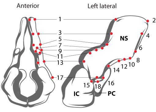
FIGURE 2. Original specimen of Acanthostega gunnari (MGUH f.n. 1227). Arrow points to neural arch of the vertebra that was used for the reconstruction.
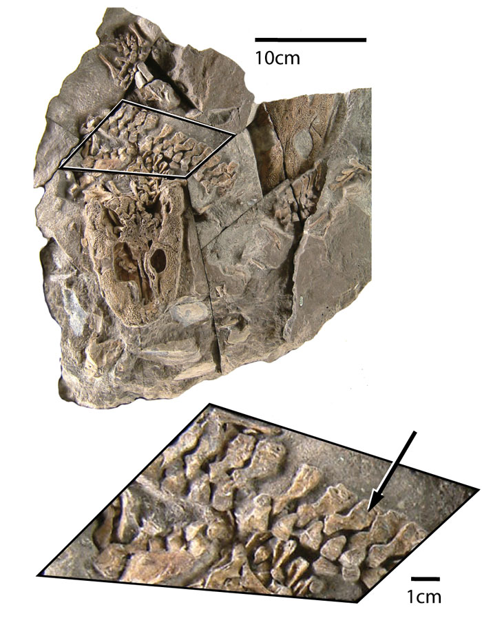
FIGURE 3. Vertebral elements segmented in Mimics from a micro-CT scan of MGUH1227. Neural spine (green), intercentrum (blue), and pleurocentrum (red) volume-rendered using the "Medium" setting (134,369 vertices). Only the left half of the vertebra is preserved, and the pleurocentrum has been taken from an adjacent vertebra.
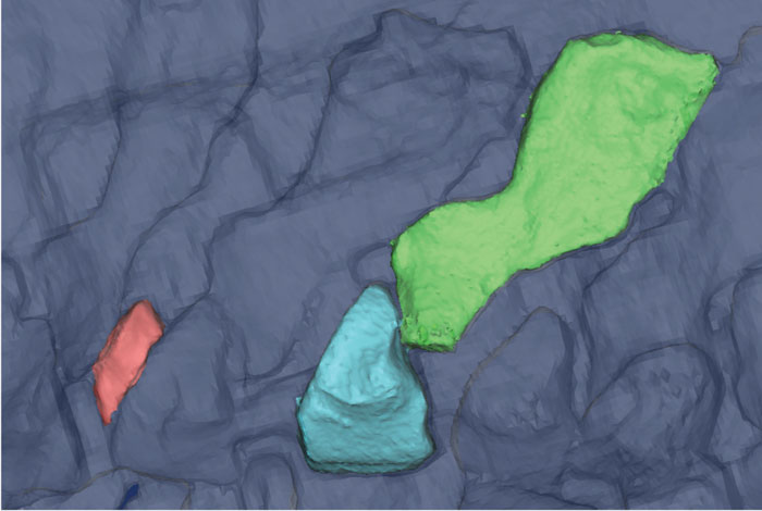
FIGURE 4. Mapping landmarks onto the scan data and planning curve placement on a neural spine of Acanthostega. 4.1, edges of major planes (blue lines); 4.2, landmarks (red dots); 4.3, perpendicular contour lines (violet); 4.4, subsidiary contour lines (green). Major plane contours define the anterior, posterior, medial, and lateral surfaces. Landmark points are located at the boundaries of major planes and structures such as neural spines, zygapophyses, and transverse processes. Perpendicular contours passing through corresponding landmark points create a grid on the surface of the template, and subsidiary contours describe the geometry of the lateral and medial surfaces of the neural arch.
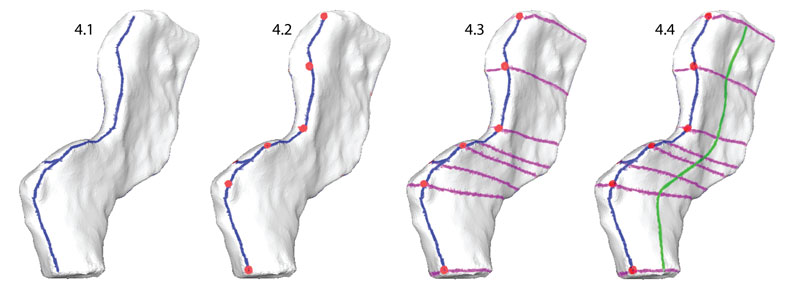
FIGURE 5. Creating contour curves. Using the Edit points curve tool, knots were placed along the contour lines (blue and green) using a setting that constrained them to the surface of the template mesh at the intersections with perpendicular lines (purple). Note that each curve has the same number of knots.
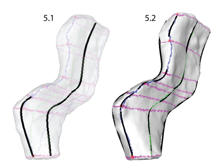
FIGURE 7. Lofting curves to create a NURBS surface. Contour curves were selected sequentially moving around the circumference of the template mesh. The curves were lofted to create the NURBS surface representing the left half of a neural spine of Acanthostega (80 knots).
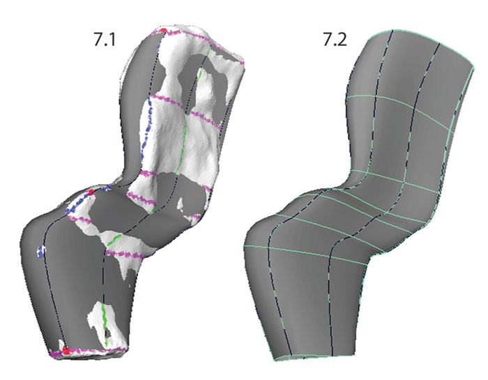
FIGURE 9. Adjusting the placement of the spline knots on the template surface. Knots were moved along the surface of the template mesh (on the left; still "Live") by dragging in the center of the Move manipulator. The NURBS surface (right) is updated automatically to reflect changes in the shapes of the curves.
FIGURE 10. Reconstruction of the medial surface using reference images. The template mesh is hidden, and the NURBS shape (grey) created from the lofted curves has been moved to the left. NURBS curves (blue) are in the center, and the reference image is on the right (Coates, 1996, figure 9c). Knots are moved using the Move tool (yellow/green arrows). The shape of the NURBS surface is updated dynamically with changes in the shapes of the curves.
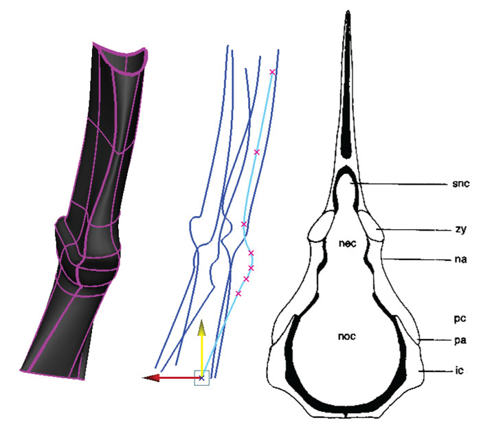
FIGURE 11. Creating the rib facet. 11.1, the curve forming the edge of the NURBS surface was duplicated twice and its pivot point was centered; 11.2, one duplicate curve was scaled to 0 and a Loft was performed between the two curves; 11.3, the resulting NURBS surface was attached to the original surface.
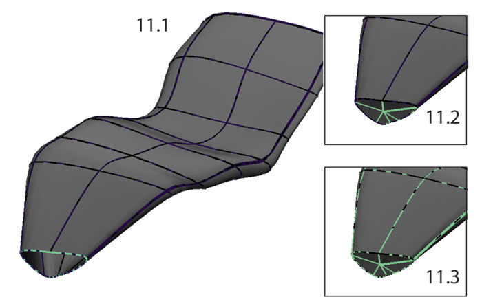
FIGURE 13. Mirroring and attaching bilaterally symmetrical elements. 13.1, neural spine, intercentrum and pleurocentrum were grouped and duplicated; 13.2, the group was mirrored across the x-axis (scaled by -1); 13.3, the intercentrum halves were attached at the midline.
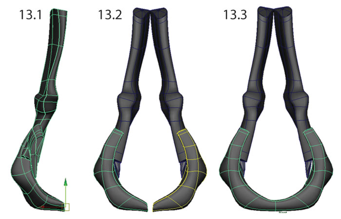
FIGURE 15. Landmarks placed for validation. 162 landmarks were used for each model: four two-point linear measurements (D1, D2, D3, D4) and six patches (P) - three on the lateral surface and three on the medial surface - composed of nine landmarks and 16 semi-landmarks each (P1-3 shown; P4-6 are on the opposite side).
FIGURE 16. Final reconstructions of a dorsal vertebra of Acanthostega. 16.1, left lateral view; 16.2, anterior view; 16.3, posterolateral view.
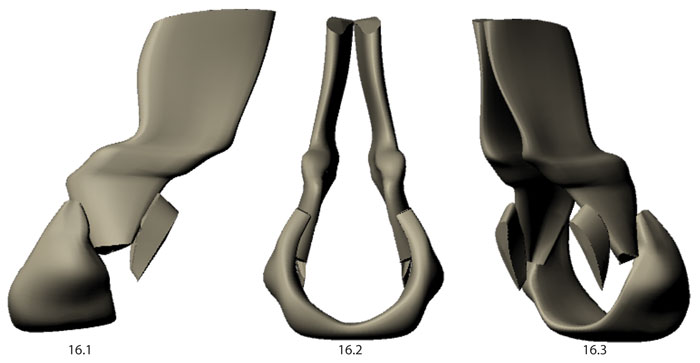
FIGURE 18. Box and whisker plot showing variation within four linear measurements taken from 15 neural arch models: D1 - neural spine width at tip, D2 - neural spine width at base, D3 - transverse process width at tip, D4 - total neural arch height.
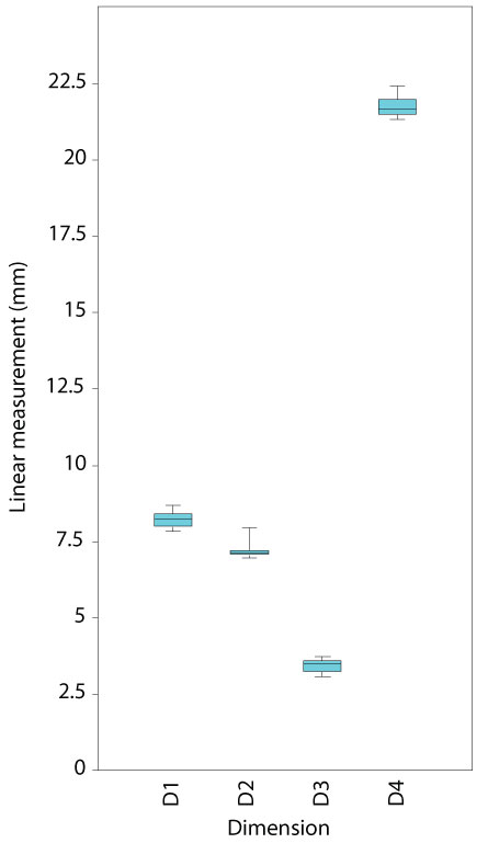
FIGURE 19. Generalized Procrustes Superimposition of landmark points showing variation in landmark position between models.
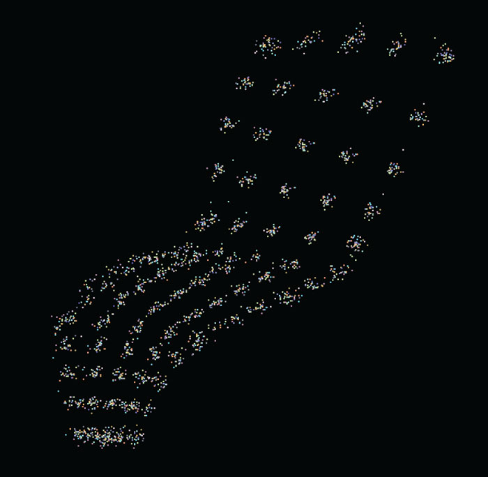
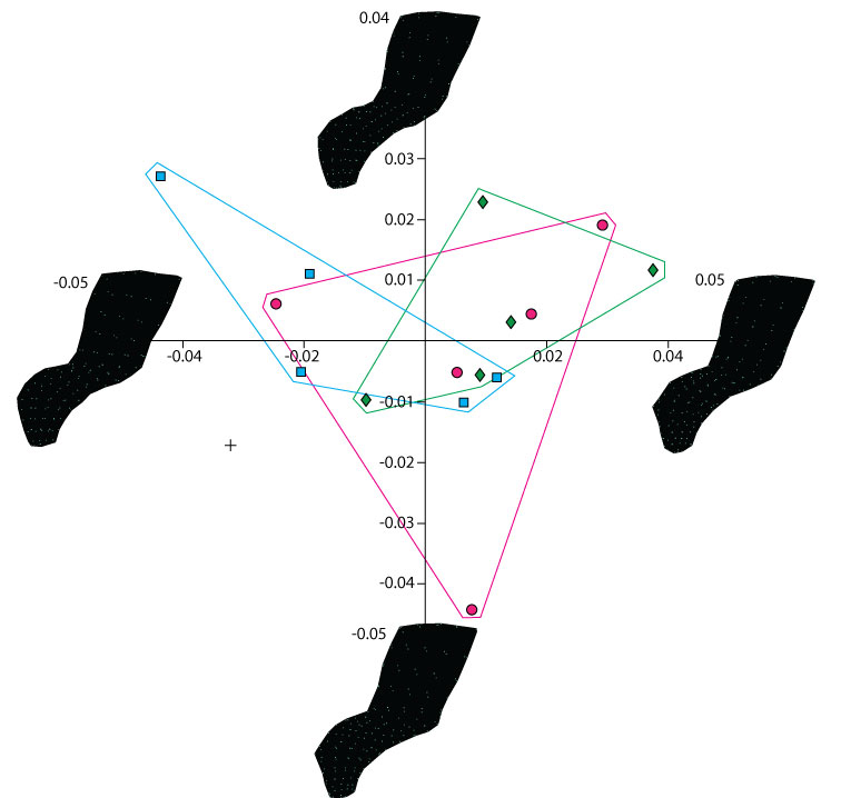
FIGURE 20. PCA showing shape differences along PC1 and PC2 between neural spine models created by different operators and the original specimen. Green diamonds represent models created by the experienced operator, blue square and pink circles the inexperienced operators and the black cross represents the original specimen. Visualization of extreme morphologies along PC1 and PC2 shows little variation between landmark configurations.