| |
MATERIALS AND METHODS
Laser Scanning and Data Acquisition
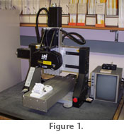 The laser scanner used in this study was a Surveyor RPS-120 probe (Laser Design Inc., Minneapolis, MN) mounted on a tri-axial automated stage (ISEL Automation, Eichenzell, Germany) (Figure 1). With this system, a red laser beam (620 nm wavelength) is emitted from the diode and spread passively into a laser plane (Figure 2.1). The laser scanner used in this study was a Surveyor RPS-120 probe (Laser Design Inc., Minneapolis, MN) mounted on a tri-axial automated stage (ISEL Automation, Eichenzell, Germany) (Figure 1). With this system, a red laser beam (620 nm wavelength) is emitted from the diode and spread passively into a laser plane (Figure 2.1).
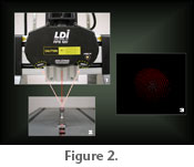 This laser plane appears as a line on the specimen and serves as the non-contact probe for the instrument (Figure 2.2). The laser line is reflected off the surface of the object and collected by dual optical sensors, charge coupled device (CCD) arrays similar to those found in digital cameras (Figure 2.1). As the stage moves the RPS (rapid profile scanning) unit over the specimen, the sensors collect a series of 2D profiles (scan-lines) of the object which collectively form a 3D coordinate point cloud of the surface (Figure 2.3). This laser plane appears as a line on the specimen and serves as the non-contact probe for the instrument (Figure 2.2). The laser line is reflected off the surface of the object and collected by dual optical sensors, charge coupled device (CCD) arrays similar to those found in digital cameras (Figure 2.1). As the stage moves the RPS (rapid profile scanning) unit over the specimen, the sensors collect a series of 2D profiles (scan-lines) of the object which collectively form a 3D coordinate point cloud of the surface (Figure 2.3).
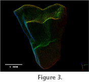 Determining instrument resolution is not straightforward, because of its unique ability to incorporate multiple views of the same specimen. Therefore, maximum resolution can only be given per scan view. A single scan has a theoretical maximum resolution of 23.0 microns along the y-axis and 27.6 microns along the z-axis, each of which are determined by the dimensions of the CCD arrays. The resolution along the x-axis is dependent on the minimum interval (step-size) of the stage stepper motor which is 10 microns. To give an idea of surface point density, the probe has the ability to collect 480 points per scan-line with point spacing of 25 microns. As an example, the minimum number of points necessary to adequately cover the occlusal surface of a marsupial molar 1.5 mm in length is around 2,500 points (Figure 3). The software used to acquire the 3D data was Surveyor Scan Control v. 4.1.009 (Laser Design Inc., Minneapolis, MN), which is an updated version of their proprietary Datasculpt software. Determining instrument resolution is not straightforward, because of its unique ability to incorporate multiple views of the same specimen. Therefore, maximum resolution can only be given per scan view. A single scan has a theoretical maximum resolution of 23.0 microns along the y-axis and 27.6 microns along the z-axis, each of which are determined by the dimensions of the CCD arrays. The resolution along the x-axis is dependent on the minimum interval (step-size) of the stage stepper motor which is 10 microns. To give an idea of surface point density, the probe has the ability to collect 480 points per scan-line with point spacing of 25 microns. As an example, the minimum number of points necessary to adequately cover the occlusal surface of a marsupial molar 1.5 mm in length is around 2,500 points (Figure 3). The software used to acquire the 3D data was Surveyor Scan Control v. 4.1.009 (Laser Design Inc., Minneapolis, MN), which is an updated version of their proprietary Datasculpt software.
Specimen Coating
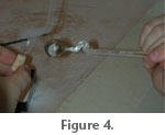 Unlike scanning electron microscopy in which high reflectivity is advantageous, the sensors in laser scanners require diffuse light. This proved especially problematic for dental specimens (or casts) because the high reflectivity of the enamel (or casting compound) caused the laser line to "shimmer" along the surface of the tooth. This created hotspots along the profile and yielded noisy point cloud data. To reduce the effects of this phenomenon, specimens were lightly dusted with an ammonium chloride (NH4Cl) coating. Other compounds were tested (i.e, Spotcheck SKD-S2 Developer, Magnaflux, Glenview, IL; magnesium chloride) but ammonium chloride proved the lightest, most efficient, and easiest to remove. To coat a specimen, the ammonium chloride was heated and vaporized in a custom built glass instrument and then mouth-blown onto the surface of the specimen (Figure 4). All specimens were dusted with the lightest possible coating, and visually examined for consistency prior to scanning. Unlike scanning electron microscopy in which high reflectivity is advantageous, the sensors in laser scanners require diffuse light. This proved especially problematic for dental specimens (or casts) because the high reflectivity of the enamel (or casting compound) caused the laser line to "shimmer" along the surface of the tooth. This created hotspots along the profile and yielded noisy point cloud data. To reduce the effects of this phenomenon, specimens were lightly dusted with an ammonium chloride (NH4Cl) coating. Other compounds were tested (i.e, Spotcheck SKD-S2 Developer, Magnaflux, Glenview, IL; magnesium chloride) but ammonium chloride proved the lightest, most efficient, and easiest to remove. To coat a specimen, the ammonium chloride was heated and vaporized in a custom built glass instrument and then mouth-blown onto the surface of the specimen (Figure 4). All specimens were dusted with the lightest possible coating, and visually examined for consistency prior to scanning.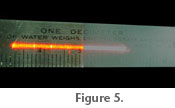 Although there is an element skill required for this method, a cautious technician can quickly learn the indications of undercoating (sparse, still semi-reflective areas; variations in color) and overcoating (thickened appearance; loss of morphological resolution). In most cases the compound can easily be dusted off with compressed air or a light brushing, and can be reapplied as necessary to achieve an even coating. As illustrated on a stainless steel scale bar, this coating was very effective in diffusing the laser light, and provided crisp reflections of the laser line (Figure 5). Beyond its diffusive effect, the specimen coating also enhanced the accuracy of the scans by yielding a consistent surface from one specimen to the next. Because variations in specimen color and texture have a profound effect on the laser's probe, the coating standardized the scan parameters and served to automate the process as well, by permitting the use of the same exposure settings for all specimens. Although there is an element skill required for this method, a cautious technician can quickly learn the indications of undercoating (sparse, still semi-reflective areas; variations in color) and overcoating (thickened appearance; loss of morphological resolution). In most cases the compound can easily be dusted off with compressed air or a light brushing, and can be reapplied as necessary to achieve an even coating. As illustrated on a stainless steel scale bar, this coating was very effective in diffusing the laser light, and provided crisp reflections of the laser line (Figure 5). Beyond its diffusive effect, the specimen coating also enhanced the accuracy of the scans by yielding a consistent surface from one specimen to the next. Because variations in specimen color and texture have a profound effect on the laser's probe, the coating standardized the scan parameters and served to automate the process as well, by permitting the use of the same exposure settings for all specimens.
Specimen Scanning and Scan Parameters
Once coated, specimens were mounted to the stage for the first of five scans. By default, occlusal view was chosen as the primary orientation of dental remains. Path plans (essentially the start and stop positions for data acquisition) were defined based on the dimensions of the specimen, and scan parameters (linear spacing and exposure) were configured. To determine the appropriate linear spacing (step-size for the stage stepper motor), multiple spacing trials (10, 20, 30, 50 µm) were conducted on isolated dental specimens of various size classes (< 4 mm in length; 4-8 mm; 8-12 mm; > 12 mm). Each resulting point cloud was examined for adequate surface coverage (point density) for the desired level of morphological resolution. The general rule developed for determining appropriate linear spacing was:
• specimens < 4 mm in length: 10 µm spacing
• specimens 4-8 mm in length: 20 µm spacing
• specimens 8-12 mm in length: 30 µm spacing
• specimens > 12 mm in length: 50 µm spacing
Because all specimens were coated with ammonium chloride, the same exposure settings could be maintained. Based on the same principal as shutter speed in photography, exposure time in laser scanning is the duration (msec) that the CCD arrays are exposed to incoming photons. Underexposure yields little or no scan data, while overexposure leads to over-saturation and thus noisy scan data. Due to variation between the two sensor arrays, it was discovered that Sensor 0 must be set to a slightly longer exposure time to acquire comparable amounts of data. With the ammonium chloride coating, the exposure for Sensor 0 was set to 0.35 msec and Sensor 1 was set to 0.25 msec. After all settings were configured, the surface point cloud data were collected and saved for a single scan orientation (view). To adequately cover the surface of a dental specimen, five views (occlusal, buccal, lingual, mesial, and distal) were typically required. The five resulting point clouds were saved as individual files, to later be registered into a cohesive model (Figure 3) during the registration process (described below).
Automation and Standardization of the Scanning and Modeling Process
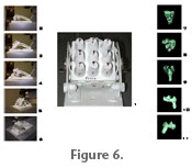 Development of the Multiscan Platform. While the aforementioned scanning procedure was effective for scanning individual specimens, in order to expedite the modeling process, it was necessary to scan and render multiple specimens simultaneously. This was accomplished by the development of a nine-specimen multi-scan platform (Figure 6.1). Because all models for PaleoView3D are complete 3D surfaces, it was necessary to adopt a rotational scanning approach to adequately cover the entire surface of the specimens. Although complete automation of the scanning process would have been possible with a manufactured motorized rotary stage, integrating it into the existing system would have been expensive (~ 10,000 USD). Additionally, with the extra stage mount, the work envelope would also have been greatly reduced. Borrowing from rotary designs of existing stages, a low-cost (< 20 USD) multiscan platform was constructed and functions as a manual version of a rotary stage. Development of the Multiscan Platform. While the aforementioned scanning procedure was effective for scanning individual specimens, in order to expedite the modeling process, it was necessary to scan and render multiple specimens simultaneously. This was accomplished by the development of a nine-specimen multi-scan platform (Figure 6.1). Because all models for PaleoView3D are complete 3D surfaces, it was necessary to adopt a rotational scanning approach to adequately cover the entire surface of the specimens. Although complete automation of the scanning process would have been possible with a manufactured motorized rotary stage, integrating it into the existing system would have been expensive (~ 10,000 USD). Additionally, with the extra stage mount, the work envelope would also have been greatly reduced. Borrowing from rotary designs of existing stages, a low-cost (< 20 USD) multiscan platform was constructed and functions as a manual version of a rotary stage.
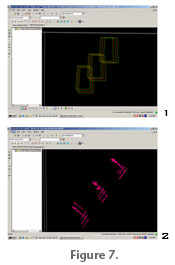 Because five views were required to adequately cover the surface of most specimens, five fixed stage positions were established (Figure 6.2-6.6). Representative scans for each corresponding position can be seen in Figures 6.7-6.11. Default path plans were defined for each stage position (Figure 7.1), automating a tedious process that can now be opened and run with a single command. Not only were the multiple specimens scanned simultaneously, the resulting nine-specimen point cloud (Figure 7.2) was imported into Geomagic Studio 6.0 and processed in unison. This bolt-on specimen holder permitted simultaneous scanning of up to nine small (< 5 mm) specimens. The nine specimen platform was chosen because the 3 x 3 design was the maximum size square that would fit within the work envelope without shading lower specimens when the stage was tilted. The stage mount and the platform (to which the specimens were affixed) were constructed of wood, and the mounting brackets were modified lid support hinge rails. Four brackets were mounted to the platform, one on each side so that it could be bolted down to the support rails at the desired angle of inclination. Standard specimen mounting corks were glued to the platform, and the mounting pins were inserted into the corks, permitting easy transfer of specimens. Because five views were required to adequately cover the surface of most specimens, five fixed stage positions were established (Figure 6.2-6.6). Representative scans for each corresponding position can be seen in Figures 6.7-6.11. Default path plans were defined for each stage position (Figure 7.1), automating a tedious process that can now be opened and run with a single command. Not only were the multiple specimens scanned simultaneously, the resulting nine-specimen point cloud (Figure 7.2) was imported into Geomagic Studio 6.0 and processed in unison. This bolt-on specimen holder permitted simultaneous scanning of up to nine small (< 5 mm) specimens. The nine specimen platform was chosen because the 3 x 3 design was the maximum size square that would fit within the work envelope without shading lower specimens when the stage was tilted. The stage mount and the platform (to which the specimens were affixed) were constructed of wood, and the mounting brackets were modified lid support hinge rails. Four brackets were mounted to the platform, one on each side so that it could be bolted down to the support rails at the desired angle of inclination. Standard specimen mounting corks were glued to the platform, and the mounting pins were inserted into the corks, permitting easy transfer of specimens.
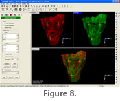 Manual Registration. Scans of all five orientations and the resulting point clouds were then imported into Geomagic Studio 6.0 (Raindrop Inc., Durham, NC) for registration (the alignment of multiple views) (Figure 8). All registrations were performed in Studio 6.0 because of a software glitch that was discovered in later versions of the program (Studio 7.0-10.0) that impaired the registration process for small (< 10 mm) specimens. This step was probably the most important of the modeling process, as it united the five scans into a single 3D point cloud. To perform the operation a minimum of three (x, y, z) points were selected on one model, and three corresponding points were selected on the second model. Points chosen were well-defined morphological structures (such as a cusp tip) that were widely dispersed on the specimen. The "Register" algorithm was applied, and the two surfaces were aligned (Figure 8). The same process was applied with this new merged object and each remaining view. Once registered, each specimen was saved individually, and subsequent operations were performed on isolated models. Manual Registration. Scans of all five orientations and the resulting point clouds were then imported into Geomagic Studio 6.0 (Raindrop Inc., Durham, NC) for registration (the alignment of multiple views) (Figure 8). All registrations were performed in Studio 6.0 because of a software glitch that was discovered in later versions of the program (Studio 7.0-10.0) that impaired the registration process for small (< 10 mm) specimens. This step was probably the most important of the modeling process, as it united the five scans into a single 3D point cloud. To perform the operation a minimum of three (x, y, z) points were selected on one model, and three corresponding points were selected on the second model. Points chosen were well-defined morphological structures (such as a cusp tip) that were widely dispersed on the specimen. The "Register" algorithm was applied, and the two surfaces were aligned (Figure 8). The same process was applied with this new merged object and each remaining view. Once registered, each specimen was saved individually, and subsequent operations were performed on isolated models.
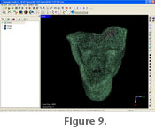 Autosurfacing Macro. Several post-registration smoothing functions (e.g., removal of outliers, uniform sampling, etc...) were performed in Studio, and the point cloud was wrapped with a polygonal surface. The processing phase of the technique was the most demanding, required the most amount of training, and was thus the largest source of human error. Any number of processing functions (e.g., Noise Reduction, Smooth, Select Outliers, etc...) can over-smooth the model and greatly alter the morphology of the specimen. To minimize error and standardize the modeling process, an autosurfacing macro was developed in Geomagic
Studio and is available for
download. Future updates may be Autosurfacing Macro. Several post-registration smoothing functions (e.g., removal of outliers, uniform sampling, etc...) were performed in Studio, and the point cloud was wrapped with a polygonal surface. The processing phase of the technique was the most demanding, required the most amount of training, and was thus the largest source of human error. Any number of processing functions (e.g., Noise Reduction, Smooth, Select Outliers, etc...) can over-smooth the model and greatly alter the morphology of the specimen. To minimize error and standardize the modeling process, an autosurfacing macro was developed in Geomagic
Studio and is available for
download. Future updates may be
available at
PaleoView3D. Creating the macro was straightforward, all desired operations and corresponding parameters were performed on an initial model and recorded in the macro as an automated file. To use the autosurfacing macro, the file is simply loaded and run with a single command, and all pre-programmed operations are applied to the current point cloud (Figure 9).
Morphometric Error Study
Because PaleoView3D models are available for public access and may be downloaded for use in morphometric applications, it was imperative that each accurately represented the original specimen. To illustrate the accuracy and precision of this new laser scanning technique, an extensive error study was performed in all three Cartesian axes. It should be noted that in each of the studies, the modeling process was repeated with consistent parameters in its entirety: coating, scanning, registration, and surface rendering (via the newly developed autosurfacing macro when applicable).
L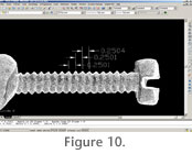 inear (1D) Error Study. Linear measurements are undoubtedly the easiest to acquire, and 1D data are still widely used in paleontological applications. Because this technique was designed for small organic specimens of various morphologies, selection of an appropriate control object was key in assessing the linear accuracy of the modeling process. A small (5.5 mm) machine tooled screw with a known thread-pitch (essentially the wavelength of the threads) of 0.250 mm was chosen as the control (Figure 10). The screw was scanned (0.01 mm linear spacing) and modeled from start to finish three separate times on independent days. Each model was composed of five scan views and rendered using the autosurfacing macro. Ten crest to crest linear measurements were taken per model using the "DimLinear" tool in AutoCAD 2005 (Figure 10). inear (1D) Error Study. Linear measurements are undoubtedly the easiest to acquire, and 1D data are still widely used in paleontological applications. Because this technique was designed for small organic specimens of various morphologies, selection of an appropriate control object was key in assessing the linear accuracy of the modeling process. A small (5.5 mm) machine tooled screw with a known thread-pitch (essentially the wavelength of the threads) of 0.250 mm was chosen as the control (Figure 10). The screw was scanned (0.01 mm linear spacing) and modeled from start to finish three separate times on independent days. Each model was composed of five scan views and rendered using the autosurfacing macro. Ten crest to crest linear measurements were taken per model using the "DimLinear" tool in AutoCAD 2005 (Figure 10).
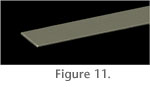 Surface Area (2D) Error Study. To incorporate the second dimension into the study, the control object chosen was a one decimeter scale bar with known dimensions of 100 x 10 x 1 mm (Figure 11). The surfaces of this scale bar were ideal for calculating the 2D area, and one long side (100 x 10 mm) was scanned and modeled three separate times. Because only a single scan view was used in model creation, the autosurfacing macro could not be utilized in this assessment. The surface area of the models was measured using the "Calculate Volumes" command in 3D-Doctor, which also yields surface area data. Since this measurement is a single command, the only source of human error is in the modeling process. Scans were maintained at the highest resolution (0.01 mm) to remain consistent with the linear error study. Surface Area (2D) Error Study. To incorporate the second dimension into the study, the control object chosen was a one decimeter scale bar with known dimensions of 100 x 10 x 1 mm (Figure 11). The surfaces of this scale bar were ideal for calculating the 2D area, and one long side (100 x 10 mm) was scanned and modeled three separate times. Because only a single scan view was used in model creation, the autosurfacing macro could not be utilized in this assessment. The surface area of the models was measured using the "Calculate Volumes" command in 3D-Doctor, which also yields surface area data. Since this measurement is a single command, the only source of human error is in the modeling process. Scans were maintained at the highest resolution (0.01 mm) to remain consistent with the linear error study.
Volumetric (3D) Error Study. The same scale bar used in the surface area study was modeled for the volumetric analysis (Figure 11). This scale bar has a known volume of 1000 cubic millimeters (100 mm x 10 mm x 1 mm). Modeling this object proved difficult due to the 1 mm thickness in the z-axis. When attempting to employ the global registration, the software would consistently attempt to register the opposing broad surfaces as a single surface. For this reason the autosurfacing macro was not used, but all steps and parameters were maintained minus the global registration. Three separate models were generated duplicating the entire process, registering six different scan views per model. The volumes were calculated in Geomagic Studio 6.0 using the "Compute Volume" analysis and cross checked in 3D-Doctor using the "Calculate Volumes" command. As with the 2D study, there was no potential source of human error in the measurement.
Casting Error Study
Because the goal of PaleoView3D is to digitize the types of Paleocene-Eocene taxa, specimens from many museums were involved in the process. Original specimens were scanned whenever possible; however, casts were also used since many museums are hesitant to loan original type material. Additionally, the type specimens of some species have been lost or damaged, so that casts are the only option. In some cases where types are lost or fragile, some museums are molding casts of earlier casts for loans. Given the use of casts for PaleoView3D scans, it was necessary to assess the accuracy of the molding/casting process. Although manufacturers publish shrinkage rates, few studies (Evans et al. 2001) have documented shrinkage rates for a single molding and casting procedure. Furthermore, there has been no assessment of the error of cumulative casting procedures. Therefore, it was necessary to examine the variation between the cast and the original specimen, as well as any "casts of casts."
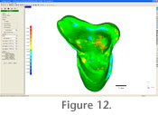 To address this issue, an isolated upper molar of an early Eocene creodont, Arfia junnei (UCMP 216155), was modeled using the laser scanning process. This specimen was then molded using Dow Corning HS III RTV Silicone and cast with TAP Plastics Four to One epoxy resin. The published shrinkage rates at 24 hours for these compounds are 0.2% and < 1.0%, respectively. This first generation cast was then scanned and rendered using the same technique. Once scanned, the molding and casting process was repeated using the first generation cast, essentially making a "cast of a cast." This process was performed twice more concluding with a fourth generation cast. Variation between the resulting models was assessed using the 3D Compare operation in Geomagic Studio 6.0. This operation generates a color-coded spectrum model illustrating areas of correspondence and deviation between the two surfaces (Figure 12). Areas of the resulting spectrum model that appear green illustrate regions of highest correspondence and in this study, deviate less than ± 0.018 mm from one another. By default, surfaces at the higher end of the spectrum (yellows and reds) highlight areas in which the second model has positive relief, i.e., is larger than the original. Those surfaces colored at the lower end of the spectrum (blues and violets) highlight areas of negative relief, or places where the second model is smaller than the original. Because the epoxy is known to shrink, some variation will be introduced simply in the alignment of the models compared. Since we were examining the effects of casting on overall morphology, we chose not to scale the models, but to compare them as produced. To address this issue, an isolated upper molar of an early Eocene creodont, Arfia junnei (UCMP 216155), was modeled using the laser scanning process. This specimen was then molded using Dow Corning HS III RTV Silicone and cast with TAP Plastics Four to One epoxy resin. The published shrinkage rates at 24 hours for these compounds are 0.2% and < 1.0%, respectively. This first generation cast was then scanned and rendered using the same technique. Once scanned, the molding and casting process was repeated using the first generation cast, essentially making a "cast of a cast." This process was performed twice more concluding with a fourth generation cast. Variation between the resulting models was assessed using the 3D Compare operation in Geomagic Studio 6.0. This operation generates a color-coded spectrum model illustrating areas of correspondence and deviation between the two surfaces (Figure 12). Areas of the resulting spectrum model that appear green illustrate regions of highest correspondence and in this study, deviate less than ± 0.018 mm from one another. By default, surfaces at the higher end of the spectrum (yellows and reds) highlight areas in which the second model has positive relief, i.e., is larger than the original. Those surfaces colored at the lower end of the spectrum (blues and violets) highlight areas of negative relief, or places where the second model is smaller than the original. Because the epoxy is known to shrink, some variation will be introduced simply in the alignment of the models compared. Since we were examining the effects of casting on overall morphology, we chose not to scale the models, but to compare them as produced.
|