Sorex morphospace dynamics

Morphospace dynamics and intraspecies variety of Sorex araneus and S. tundrensis according to recent and fossil data

Leonid L. Voyta, Evgeniy P. Izvarin, Yulia A. Shemyakina, Viktoria A. Nikiforova, Tatyana V. Strukova, Nikolai G. Smirnov, Daniel A. Melnikov, and Anatoly V. Bobretsov

Article number: 26.3.a51
https://doi.org/10.26879/1330
Copyright Paleontological Society, December 2023

Author biographies
Plain-language and multi-lingual abstracts
PDF version

Submission: 17 August 2023. Acceptance: 9 November 2023.

ABSTRACT

Several patterns were revealed in a temporal study on morphological variety of Sorex araneus and S. tundrensis (Soricidae, Mammalia). We examined samples from 18 modern and three fossil Early-Late Holocene Uralian localities. We analyzed shape variation of the first lower molar and hemimandible using two-dimensional geometrical landmarks; size differences were estimated by means of three linear measures. A separate purpose was estimation of the measurement error that arose during the data acquisition. We found that the modern samples of both species share underestimated similarity in both size and shape of morphological structures. Regression analysis revealed different phenotypic traits of the mandibular proportion in the large and small shrews regardless of species attribution. A size decrease of S. araneus and conversely a size increase of S. tundrensis both drive the mandibular shape toward phenotypic convergence. This pattern, however, is violated in the fossil samples, where the largest S. tundrensis from a Late Holocene Sim III locality (South Ural) showed a well-distinguishable mandibular shape located in a separate part of the morphospace. In this work, we found that the m1 shape has only weak resolving power as compared to the mandibular or especially skull shape. Nonetheless, even the moderate resolving power of the mandibular shape allowed us to uncover phenotypic changes during the Holocene that have not been noticed by previous researchers at Uralian late Quaternary localities.

Leonid L. Voyta. Zoological Institute (ZIN), Russian Academy of Sciences, Universitetskaya nab. 1, Saint Petersburg, 199034, Russia. leonid.voyta@zin.ru
Evgeniy P. Izvarin. Institute of Plant and Animal Ecology (IPAE), Ural Branch, Russian Academy of Sciences, 8 Marta St. 202, Yekaterinburg, 620144, Russia. izvarin_ep@ipae.uran.ru
Yulia A. Shemyakina. Zoological Institute, Russian Academy of Sciences, Universitetskaya nab. 1, Saint Petersburg, 199034, Russia. julia.shemyakina@zin.ru
Viktoria A. Nikiforova. Zoological Institute, Russian Academy of Sciences, Universitetskaya nab. 1, Saint Petersburg, 199034, Russia. victoria.nikiforova@zin.ru
Tatyana V. Strukova. Institute of Plant and Animal Ecology, Ural Branch, Russian Academy of Sciences, 8 Marta St. 202, Yekaterinburg, 620144, Russia. strukova@ipae.uran.ru
Nikolai G. Smirnov. Institute of Plant and Animal Ecology, Ural Branch, Russian Academy of Sciences, 8 Marta St. 202, Yekaterinburg, 620144, Russia. nsmirnov@ipae.uran.ru
Daniel A. Melnikov. Zoological Institute, Russian Academy of Sciences, Universitetskaya nab. 1, Saint Petersburg, 199034, Russia. daniel.melnikov@zin.ru
Anatoly V. Bobretsov. Pechora-Ilych State Nature Reserve, Laninoy Str. 8, Yaksha Village, 169436, Komi Republic, Russia. avbobr@mail.ru

Keywords: Soricidae; Sorex; paleocommunity; morphospace dynamics; Holocene; geometric morphometrics

Final citation: Voyta, Leonid L., Izvarin, Evgeniy P., Shemyakina, Yulia A., Nikiforova, Viktoria A., Strukova, Tatyana V., Smirnov, Nikolai G., Melnikov, Daniel A., and Bobretsov, Anatoly V. 2023. Morphospace dynamics and intraspecies variety of Sorex araneus and S. tundrensis according to recent and fossil data. Palaeontologia Electronica, 26(3):a51.
https://doi.org/10.26879/1330
palaeo-electronica.org/content/2023/4024-sorex-morphospace-dynamics

Copyright: December 2023 Paleontological Society.
his is an open access article distributed under the terms of Attribution-NonCommercial-ShareAlike 4.0 International (CC BY-NC-SA 4.0), which permits users to copy and redistribute the material in any medium or format, provided it is not used for commercial purposes and the original author and source are credited, with indications if any changes are made.
creativecommons.org/licenses/by-nc-sa/4.0/

INTRODUCTION

Long-term biotic responses to past climate change are the key aspect of assessment of the stability of animal and plant communities and are usually poorly applicable to the analysis of recent environments. Even the longest-standing monitoring systems (e.g., the Flathead Lake Biological Station in the USA since 1899 and the Pacific Biological Station in Canada since 1908) cover relatively short time spans compared to the shortest periods of global climate fluctuation that can be identified by analytical or instrumental methods in the history of the Earth (deMenocal et al., 2000; Kotthoff et al., 2008). In this context, studies on paleocommunities are becoming increasingly important (Jackson and Blois, 2015; Andermann et al., 2020), while community dynamics and spatial fluctuations during and between global and regional environmental crises have gained popularity for predicting the state of modern communities (e.g., Willis et al., 2010; Jackson and Blois, 2015).

One feasibly useful set of fossil records are preserved remains of small-mammal communities in loose cave sediments of the late Quaternary of the Palearctic and Nearctic. The uniqueness of these records is determined by the continuity of communities from at least the Late Pleistocene to modern times. In several studied regions of the North Palearctic during late Quaternary spatial fluctuations of glacial and interglacial biomes, there is continuity between paleo- and modern communities of small mammals (Zaitsev and Osipova, 2005; Fadeeva, 2016; Smirnov et al., 2016; Baca et al., 2017, 2020; Omelko et al., 2020; Izvarin et al., 2022; and many others).

Usually, in the investigation of the paleocommunities, preference is given to rodents, which form the basis of biostratigraphy (Agustí, 1999; Daxner-Höck et al., 2013; Koufos, 2013; Ponomarev and Andreicheva, 2019; Martin and Kelly, 2023). On the other hand, shrew communities are also suitable as a rich source for the analysis of biotic responses, including changes in morphometric traits (Reumer, 1984; van Dam, 2004; Furió et al., 2007, 2018; Furió and Agustí, 2017). Although shrews have special value, their morphometric study usually reaches either a single-species analysis (Panasenko and Kholin, 2011; Polly, 2005, 2007; Voyta et al., 2013; Cornette et al., 2015a; Rofes et al., 2018) or an analysis of univariate/bivariate statistics (Fadeeva, 2016; Zazhigin and Voyta, 2018; Moya-Costa et al. 2023). Currently, there are not many comprehensive studies on the morphometric variety of shrews on a multispecies scale (Butler et al., 1989; Zaitsev, 1998; Dokuchaev et al., 1999, 2010; Zazhigin and Voyta, 2022), especially used powerful geometric morphometric approaches based on two- and three-dimensional data sets (Rychlik et al., 2006; Cornette et al., 2015a, 2015b), various methods of interpretation (e.g., multivariate shape space approach; Polly and Wójcik, 2019) and molecular/morphological data sets combining (Voet et al., 2022), although, other mammalian groups are being developed very actively (Hulme-Beaman et al., 2019; Terray et al., 2022; Viacava et al., 2023; and many others).

Modern soricids (Soricidae, Eulipotyphla) form highly diverse species associations. They have the highest species diversity in tropical and subtropical zones, which is reached mostly by white-toothed crocidurine shrews (see overview by Dudu et al., 2005; Happold and Happold, 2013), whereas in temperate and polar zones, high species diversity is mostly shown by red-toothed soricine shrews (Zaitsev et al., 2014; Burgin and He, 2018). This trend has lasted from the Late Pleistocene, at least for many known Late Pleistocene sites of the Palearctic, where Sorex (Linnaeus, 1758) species have dominated (Zaitsev and Osipova, 2005; Fadeeva, 2016; Smirnov et al., 2016; Omelko et al., 2020). In fact, one of the richest shrew communities is composed of 12 species, has lived in East Asia since the late Quaternary period, and exceeds species diversity of arvicoline cricetids, composed of only eight species (Omelko et al., 2020). Because of the endemism, some shrews are considered environmental indicators, e.g., Crocidura sp. at Uralian fossil sites (Zaitsev, 1998), or Sorex mirabilis Ognev, 1937, at Russian Far Eastern sites (Omelko et al., 2020). According to studies by Polly (Polly, 2005, 2007; Rychlik et al., 2006; Polly and Wójcik, 2019) and Cornette (Cornette et al., 2013, 2015a,b), late Quaternary climatic changes should have influenced the composition of communities and the morphology of species, with marked cooling and warming fluctuations. It is widely accepted that the moderate environmental influence can determine changes in the overall size of shrews, usually in contradiction to Bergmann’s rule, which means that cooling causes a size decrease, whereas warming a size increase (Carraway and Verts, 2005; Rychlik et al., 2006; Panasenko and Kholin, 2011; Omelko and Kholin, 2017), as assumed in accordance with consequences of a composition of the trophic niches (Churchfield, 1994; Hanski, 1994). Nonetheless, we only vaguely know how separate or covariate morphometric features change within a community of coexisting species between cooling and warming periods, or in the spatial sense, between North and South samples.

In this context, especially interesting is the geographically and ecologically wide-ranging common shrew, Sorex araneus Linnaeus, 1758, that has usually found in most Upper Pleistocene and Holocene cave deposits of Europe, of the Russian Plain, and of the Urals (Zaitsev, 1992, 1998; Rzebik-Kowalska, 1998, 2006; Fadeeva and Smirnov, 2008; Agadjanian, 2009; Fadeeva, 2016; Izvarin et al., 2020, 2022; and many others).

The common shrew is the most popular research subject in different aspects of evolutionary biology, adaptation, and speciation (see reviews by several authors, e.g., Shchipanov et al., 2014; Polly, 2019; Thaw et al., 2019; Taylor et al., 2022) just as the house mouse model (Zima and Searl, 2019). Intensive investigations in the last three decades have revealed high levels of phenotypic and genotypic polymorphisms among recent samples of the common shrew (Searle and Wójcik, 1998; Polly, 2003, 2005, 2007; Wójcik et al., 2003; Mishta and Searle, 2019; White et al., 2019; Zima and Searl, 2019). To date, 76 chromosomal races have been described (Bulatova et al., 2019), which have been combined into several karyotypic groups. These groups partly match the phylogeographic groups revealed by analyses of mitochondrial gene cytb (Thaw et al., 2019). Both the karyotypic and phylogenetic diversification of groups were affected by Late Pleistocene and Holocene climatic events (Thaw et al., 2019; White et al., 2019). On the other hand, morphometric analyses of geographic samples have yielded inconsistent results, i.e., in several articles, morphometric variation usually contradicts individual race boundaries (Searle and Thorpe, 1987; Wójcik et al, 2000; Banaszek et al., 2003; Mishta, 2007), but in several reports, the morphometric variation correlates with karyotypic group compound (Chętnicki et al., 1996; Polyakov et al., 2002). In addition, the discussion of inter- and intragroup differentiation covers the mosaicism of morphometric differences in agreement with Pleistocene and Holocene glaciation events (Polly, 2019; Thaw et al., 2019; White et al., 2019). Therefore, the high intraspecific variety and high abundance in the late Quaternary fossil records have made this species the most suitable model for the analysis of different levels of morphometric variety and for assessing magnitudes of variation.

On the other hand, investigations of the modern morphometric variation do not always allow us to resolve a “temporal variation” and to figure out which species or probably which unknown form we are dealing with. In this regard, we have many examples from application of the open nomenclature (e.g., Sorex aff. araneus, Sorex cf. araneus; see Rzebik-Kowalska, 1998: 56) for clear-cut re-identification of a fossil material by “ancient DNA” analysis (Prost et al., 2013). The latter case is very revealing and considers significant differences in size between the fossil forms that have been assigned the species status, namely, S. araneus vs. fossil species Sorex macrognathus Janossy, 1965. Both species, despite differences in morphometric features, have formed a monophyletic clade (Prost et al., 2013).

In this work, we studied the intraspecific variation of dental and mandibular features of the common shrew, as the most abundant components of the fossil records, by geometric morphometrics and via the morphospace approach to assess the magnitude of variation at different levels, from race to geographic samples. This became possible due to a rich zoological collection of modern (ZIN) and fossil (IPAE) datasets on the common shrew. In addition, some of the datasets were already used in a published study by Shchipanov et al. (2014), and the current study addresses the supposedly “mixed” nature of some samples of S. araneus used there (Manturovo and Pechora chromosomal races). Accordingly, next, we tried to resolve the issue of mixed samples by adding modern samples of Sorex tundrensis Merriam, 1900. The main purpose of the study was to provide an update on the morphometric variation of S. araneus and S. tundrensis from three late Quaternary North, Middle, and South Ural localities.

Institutional abbreviations. IPAE: the Institute of Plant and Animal Ecology, the Ural Branch of the Russian Academy of Sciences, Yekaterinburg, Russia; IVPP: the Institute of Vertebrate Paleontology and Paleoanthropology, the Chinese Academy of Sciences, Beijing, China; ZIN: the Zoological Institute of the Russian Academy of Sciences, St. Petersburg, Russia.

MATERIAL AND METHODS

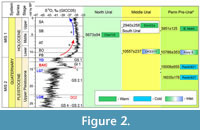
The material of Sorex araneus investigated in this work comprises 281 specimens, of which 259 come from eight recent localities (Figure 1; Appendix 1), and 22 fossils from three Holocene localities: Cheremukhovo-1 Cave (Cher1; MIS 1; Strukova et al., 2006), the North Urals; Dyrovatyi Kamen' Grot, layer 11 (DKS3/11; MIS 1; Smirnov, 1993; Ulitko, 2006), the Middle Urals; and Sim III Cave, layer 2a (Sim3/2a; MIS 1; Smirnov et al., 1990), the South Urals (Figure 2; Appendix 2). The recent samples include three samples of the Serov chromosomal race (“Valley,” “Foothill,” and “Hill”) and one sample of the Pechora race (“Ulashevo”; Appendix 1), earlier analyzed by Shchipanov et al. (2014).

During preparation of the material that was subsequently published by Shchipanov et al. (2014), in 2012, Dr. Nikolay E. Dokuchaev divided the sample of the Manturovo race into S. araneus and partly S. tundrensis subsamples. Therefore, Shchipanov et al. (2014) analyzed only the former subsample. In the current study, we analyzed the second subsample of the Manturovo race, and this task required that we include a reference sample of S. tundrensis. Thus, the material of S. tundrensis investigated in this work comprises, together with the subsample of the Manturovo race (n = 12, re-attributed to S. tundrensis), 40 specimens, of which 31 come from 10 recent localities (Figure 1; Appendix 1) and nine fossils from DKS3/11 layer (Figure 1 and Figure 2; Appendix 2).

Information about the Fossil Samples and ¹⁴C Dating

The age of the fossils used in this analysis was taken from published sources: Smirnov et al. (1990), Smirnov (1993), Ulitko (2006), and Strukova et al. (2006). The information on the Pre-Uralian localities that were included in univariate comparisons of measurements came from the study by Fadeeva (2016).

(Cher1) Cheremukhovo-1 Cave: Rock Massif Chertovo Gorodishche on the right bank of the Sos'va River, the North Urals. Collector Dr. Tatyana V. Strukova (Strukova et al., 2006): (Cher1/4), quadrat D/3, layer 4; (Cher1/4-5), quadrat D/3, layers 4-5; (Cher1/5), quadrat D/3, layer 5, horizon 45-65 cm (5673 ± 94 calibrated years before the present [cal BP]). Based on the spatial relation of the layers, we conventionally assumed that Cher1/4 and Cher1/4-5 have the same age as Cher1/5 does (Figure 2: Cher1/5).

(DKS) Dyrovatyi Kamen' Grot: Ser'ga River, the Middle Urals. Collector Prof. Nikolay G. Smirnov; collected in 1992 (Smirnov, 1993; Ulitko, 2006): (DKS3/11), layer 3, quadrat E/8, horizon 11 (10557 ± 234 cal BP).

(Sim3) Sim III Cave: Sim River, the Middle Urals. Collector Prof. Nikolay G. Smirnov (Smirnov et al., 1990): (Sim3/2а), layer 2a (lens within 2b layer), depth 5-15 cm (2940 ± 258 cal BP).

The calibrated dates have been obtained through the intCal20 Curve (Reimer et al., 2020; Appendix 2: Table A2-1). The geochronology of the Late Pleistocene and Holocene used for preparing Figure 2 was taken from the GICC05 Project (Andersen et al., 2006; Rasmussen et al., 2006; Svensson et al., 2008) and climate-stratigraphic units from refs. (Bond and Lotti, 1995; Lisiecki and Raymo, 2005; Rasmussen et al., 2014; Railsback et al., 2015).

Geometric Morphometrics and Linear Measurements

The first lower molar, m1 (just as teeth in general), is the most common of fossil remains; accordingly, the preliminary idea behind this study was to implement m1 shape analysis for precise determination of shifts/trajectories in the morphometric features between the “Cold” and “Warm” late Quaternary intervals. Nonetheless, a mixed sample from the Dan' village (Appendix 1: 10) and the presence of S. tundrensis (Appendix 2) in the fossil material forced us to extend the datasets for more reliable species identification. Hence, in the current analyses, we used two morphological complexes: (i) the first lower molar in the occlusal projection in a manner like that of Shchipanov et al. (2014); and (ii) the hemimandible in the medial projection.

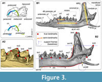Hemimandible and tooth shapes were captured as sets of two-dimensional (2D) coordinates composed of 48 and seven landmarks, respectively. The shape of m1 is described by seven true landmarks (Polly, 2007; Shchipanov et al., 2014) that are located at tips of the conids and bends of the lophids (Figure 3A; Appendix 3: Table A3-1). The hemimandible is described by six true landmarks (types I and II sensu Bookstein, 1991), together with 45 semilandmarks (Figure 3B; Appendix 3: Table A3-2). True and semilandmarks were processed using the tpsDig2 software ver. 2.31 (Rohlf, 2007), the latter together with tools “Draw background curves” and “aligning of the curve,” and support frames (“baselines”) as described by Voyta et al. (2021). The support link and slider files for analysis of the semilandmark dataset were prepared in the tpsUtil software ver. 1.28 (Rohlf, 2004). The Procrustes superimposition procedure and principal component analyses (PCAs; “relative warp analyses”) were performed by means of the tpsRelw software ver. 1.35 (Rohlf, 2003). PCA was based on the “Procrustes coordinates” (the Cartesian coordinates of each landmark after the Procrustes fitting procedure; see Rohlf and Slice, 1990).

The hemimandible dataset was reduced in size in comparison to the m1 dataset using the rarefaction approach. We reduced samples of the Serov race because there is no doubt about their species assignment (see details below). Therefore, from each sample, we randomly chose 15 specimens. The rarefaction was executed in Microsoft Excel by means of a random-number generator. Other samples were unreduced. The mandibular dataset (recent) consisted of 138 specimens; the m1 dataset (recent) was composed of 273 specimens.

In fact, the size parameter plays a substantial role in species diversification, especially in shrew communities, due to the trophic niche aspects in the sense of Hanski (1994). In the current study, using the “Snipping Tool” for Windows OS (Microsoft) for speeding up image processing (see details in Appendix 3), we replaced the usual “centroid size” with absolute dimensions in millimeters. The choice of the dimension set was based on publications of Zaitsev (1998) and Fadeeva (2016) and involved three linear characteristics: lingual length of m1 (Lm1), mandibular ramus height (MRH), and “lower molars’ length” (aLML), i.e., alveolar length of the lower molar row (Figure 3B).

In addition, parameter Lm1 was measured twice: first, via three-dimensional (3D) models using the “Measurement Tool” of Avizo 2019.1 (FEI SAS), and second, by means of 2D images of the medial view of the hemimandible in the tpsDig interface.

The Morphospace Approach and Measurement Error

In this work, the morphospace approach (Wills et al., 1994; Eble, 2000; see details in Voyta et al., 2021) was employed both for measurement error (MEr) assessment and for evaluation of inter- and intraspecies variety.

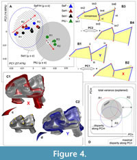In the case of difficulties with a specimens positioning, for example, during acquisition of 2D occlusal shape of m1, we encountered the issue of repeatability, when the error of positioning (orientation error, MEr) could be like or greater than intergroup differences. Usually, this issue is resolved by the repetition of the elemental operation with subsequent averaging of corresponding values (Polly, 2003). In a similar manner, we prepared three replicate datasets for each analyzed sample and assessed the size of differences between the replicates in comparison to differences between original shrew samples. In the morphospace sense all assessments were based on a variance range. For the calculation of MEr, we summed the variance of each replicate along “significant” principal components (see below). The subsequent procedures included determination of (i) the mean of the variance range of the replicates and (ii) the maximal deflection value of the replicates per sample (Figure 4D). The values of variance (general vs. each group) were calculated in the PAST software ver. 2.04 (Hammer et al., 2001; “Univariate/Summary statistics”) for principal component scores. The total value of MEr (MSMEr, morphospace measurement error estimation approach) within an appropriate morphospace/dataset was defined as the sum of all values of disparity between means of each sample (mean _(repA-C)) and the maximal value among replicates (max _(repn)):

MEr = sum MEr _(PC1-PCn) = (A mean _(repA-C) ² - A max _(repn) ²) + (N mean _(repA-C) ² - N max _(repn) ²) + <...>

where A, N, <...> are specific samples that constituted the morphospace.

According to the loading of the principal components (% of variance), we calculated a proportion of the variance (%) representing measurement error (Table 1).

During a discussion of the different approaches to measurement-error estimation (including MSMEr and Intraclass Correlation, ICC, by Bartlett and Frost, 2008) with Dr. Andrey Yu. Puzachenko, he proposed that we use a “more common” approach based on ANOVA, for example, Variance Components Approach (Prins et al., 2012). Therefore, we performed the estimation of variance components in Statistica 64 software ver. 10 (StatSoft). The calculation was based on the m1 dataset for four samples and three replicates (similarly to MSMEr estimation). The estimation was carried out by means of two factors and their interaction: “Sample” vs. “Replicate.” The estimation method was ANOVA. The results are represented in Table 2 and Appendix 4.

Imaging, 3D Models, and Visualization

The first shape analysis of m1 of shrews from the Serov and Pechora chromosomal races was carried out by Shchipanov et al. (2014). In that study, m1 images were obtained by means of a digital camera combined with a binocular microscope (Leica MZ6). To avoid the influence of MEr, in accordance with Polly (2003) recommendations, those authors implemented five replicates of separate acquisition of images. In the current study, we replaced the image acquisition using a microscope by the acquisition of images directly from 3D models. The latter approach allows to reveal the key points of the correct/repeatable tooth alignment and to control this procedure through an application interface (e.g., MorphoDig; Appendix 3: Figures A3-2 and A3-3). We admit that this approach is easier than alignment of physical specimens under a microscope, with one main limitation being availability of 3D models. In this work, we prepared 3D models of hemimandibles of the following samples: SeV (n = 59), SeF (75), SeH (63), PtU (56), S. araneus form the geographic ranges (n = 5), S. tundrensis (6), a subsample of Manturovo (9), fossil specimens of S. araneus (n = 7), and fossils of S. tundrensis (3) (see Appendix 1 and Appendix 2). All models in the PLY format are available via MorphoBank Project 4500.

Three-dimentional models were obtained on a NeoScan N80 X-ray computed micro-tomographic scanner at the core facility Taxon (http://www.ckp-rf.ru/ckp/3038/) of the Zoological Institute of the Russian Academy of Sciences (Saint Petersburg, Russia). Spatial resolution of the specimen scans ranged from 6.00 to 7.30 μm. For reducing the scanning time per specimen, we used a “specimen conglomerator” (Appendix 3: Figure A3-4), which allows to save time by simultaneous scanning of four hemimandibles instead of one. A “segmenting” of specimens within common volume was performed using DataViewer software ver. 1.5.4.0 64-bit (SkyScan, Brucker microCT) and the “Draw/Save Multiple Volume of Interest (VOI)” tool, which helps to extract each specimen as a separate part.

Contrary to the difficult orientation of m1, the hemimandible orientation is a relatively simple action due to the overall flat shape of the lateral side of the mandible. Two-dimentional hemimandible images in the medial view were captured with a Canon 60D digital camera combined with a Canon EF-S 60mm f/2.8 Macro USM lens and two flashes Godox TT350C. Each image included a scale bar.

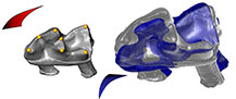
Visualization of m1 and hemimandible shape transformations between S. araneus and S. tundrensis was performed using statistical and graphical R-packages: Morpho (Schlager, 2017) and RGL (Adler and Murdoch, 2021). The visualization approach that was implemented earlier for shrew morphological description is described by Voyta et al. (2022a, 2022b).

Statistics

The Procrustes superimposition procedure and PCA of the m1 dataset were conducted with the MorphoJ software ver. 1.06d (Klingenberg, 2011); the calculation of the shape variables for the hemimandible dataset was performed in tpsRelw (see above).

For finding a possible interaction between linear measurements within S. araneus and S. tundrensis, we implemented an approach to the fitting of observed data to the von Bertalanffy growth model (Hammer et al., 2001: 5). This model can show a “bend” of a regression line; in this case, we applied bivariate linear regression to each part of the von Bertalanffy model line. Both calculations were executed with the PAST software, ver. 2.04 (Hammer et al., 2001).

To search for a gap between values of the linear characteristics, we used “Homogeneity Tests” (e.g., the Shapiro-Wilk normality test in PAST; see Hammer et al., 2001).

The number of loaded principal components (the number of the “significant” principal components) was determined using the broken-stick model with 1000 bootstrap replicates (Jackson, 1993; Hammer et al., 2001). The components located above the “broken-stick” were chosen for the analysis. This approach allows us avoid possible misinterpretations of the morphospace analysis on the basis of PCA, which were discussed in the recent paper of Polly (2023).

RESULTS

Measurement-error Estimation

Datasets of m1 were prepared during a relatively long period from February to June 2023. Nonetheless, we tried to complete the sample processing within a short period, i.e., we landmarked three replicates of a given sample at intervals of 2-3 days. Consistently with this relatively “slow” work, we revealed different directions (trajectories) of MEr formation (Figure 4A). Samples of the Serov race (SeV, SeF, and SeH) were prepared during a shorter period as compared to the Pechora race sample (PtU); therefore, Figure 4A shows the same MEr trajectory for Serov and an orthogonal trajectory for Pechora. Broad variance of the centroid of replicates in the space of the first two principal components (PC1 loading was 27.41%, and that of PC2 14.89%) revealed instability of the replicates. Nevertheless, we can see notable differences between centroids of replicates of the grouped Serov samples and of the separate PtU sample, both along PC1 and along PC2 (see unreduced variance in Appendix 4: Figure A4-1). For the visualization of the variance, we added confidence intervals based on standard deviations (SD) of each sample mean (μ ± σ). Each interval represents a predicted variance of approximately 68% of the sample around the mean. Thus, we can see differences between samples by means of the confidence interval overlap: SeF/SeH differ more strongly from PtU in the m1 shape than SeV; among the Serov samples, we revealed only small differences.

Shape differences along PC1 included (Figure 4: B1 vs. B2) at least four points: (i) well-pronounced paralophid bending (stronger in Serov than in PtU); (ii) oblique anteroposterior shifting of the protoconid tip (more posterior location in Serov than in PtU); (iii) lingual protrusion of the metaconid tip (more lingual location in Serov than in PtU); (iv) in contrast to “ii,” oblique anteroposterior shifting of the hypoconid tip (more anterior location in Serov than in PtU). The differences along PC2 included (Figure 4: B3 vs. B4) three added points: (v) anterior shifting of the paraconid and (vi) posterior shifting of metaconid, together determining differences in the trigonid length (longer at the positive end of PC2 and shorter at the negative end); (vii) some convergence of the hypoconid and entoconid tips that forms a narrow (positive end of PC2) and wide (negative end of PC2) talonid. It should be noted that all the presented differences (Figure 4B) are exaggerated for visualization purposes; in actuality, the differences between intraspecies samples were not so pronounced.

A simulation of the tooth orientation with the help of 3D models (Figure 4C) allowed us to suppose that some of the described shape differences (at least i-v) could be explained by the orientation error of m1 during the preparation of the images. Because the confidence intervals of the Serov and Pechora samples overall overlapped narrowly, we hypothesized the existence of an underestimated proportion of original differences between samples.

For revealing the proportion of “original” differences between samples and “artificial” differences produced by MEr, we first implemented the MSMEr approach, and second, variance components estimation. Table 1 shows variances of the four samples in terms of the replicates judging by the four principal component scores. We utilized the broken-stick model (Jackson, 1993) for determining the number of “loaded” principal components and thus identified the first four components as loaded with meaningful information (i.e., components that are responsible for 66.26% of explained variance). For the MEr calculation, we used disparity between variance of the most outlying replicate and a specific samples variance; the disparity was calculated from mean values, and therefore for four samples and four components, we obtained 16 disparity values, each representing MEr because it showed the most fluctuation in tooth orientation. Translation of this value to the variance proportion in percentages enabled us to estimate the MEr size in relation to the explained variance along each principal component. According to the results of this approach, the portion of MEr within PC1-4 was 30.69%, i.e., the orientation error constitutes about half of the variance, and the other half describes differences proper between the analyzed samples. This finding allowed for separate original and artificial differences, but we supposed the presence of an underestimated portion of MEr variance (within 30.69%) related to a possible interaction between samples and replicates that is shown by different trajectories: “a” and “b” (Figure 4A).

Table 2 presents results of the variance components analysis with ANOVA estimation for the same samples, replicates, and axes as described for Table 1. The estimation was performed with two factors and their interaction: “Sample” vs. “Replicate.” The former was statistically significant for all given components (F = 6.21-97.16); the factor “Replicate” was also significant for the first three components, and besides, its impact in PC1 variance was larger than that of “Sample” (MS = 0.028 vs. 0.024; F = 110.52 vs. 97.16; Table 2). The factors interception was statistically significant for the first three components thus confirming the underestimated portions of variance related to the original and artificial differences and their interaction. According to the results of this approach, the proportion of MEr within PC1-4 was 19.24% of the total variance, the original differences between samples constituted 28.84%, and interception effects were responsible for 16.05%. The variance components analysis more precisely revealed the variance distribution between specific effects than MSMEr did. Based on the results of the MEr estimation, further analyses of the m1 shape differences were executed using mean values calculated from three replicates.

Interspecies Shape/size Differences

The main issue with MEr estimation was related to assessing the intraspecies magnitude of the shape differences. The investigation gave a satisfactory result, where two geographical samples of S. araneus, Serov and Pechora, differed in the m1 shape. Then, in the context of the shape difference evaluation, we needed to expand the list of samples with the sample from Dan', composed of S. tundrensis and original S. tundrensis samples (Appendix 1).

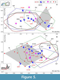A combined PCA of the recent samples of S. araneus and S. tundrensis yielded an unexpected result: the differences in the m1 shape between S. araneus samples have approximately the same order of magnitude as differences between S. araneus/S. tundrensis samples (Figure 5A). The Pechora convex hull almost fully overlapped with the convex hull of S. tundrensis. Besides, Dan' sample within the PC1-2 space is divided into three parts: a part with S. tundrensis (the positive end of PC1), a part within the PtU convex hull (the middle part of PC1), and a part outside the PtU convex hull (negative values of PC1). This finding raises the main question: What is the nature of PtU? We can theorize the presence of S. tundrensis within PtU; this presence, however, was not revealed by Shchipanov et al. (2014).

To resolve this issue, we performed a shape analysis on the skull of samples of interest: PtU and Dan', together with two reference samples of S. araneus (SeV) and original geographical samples of S. tundrensis. The results revealed a clear-cut difference between S. araneus and S. tundrensis that is related to the overall skull ratio of lengths of rostral and braincase parts (Appendix 5: Figure A5-1). The whole PtU sample, except for a single specimen (ZIN 107849/1063), was associated with S. araneus. The Dan' sample was divided partly into S. tundrensis (ZIN 107852/727, /957, /1089, /1129, /1182, and /1221; n = 6) and partly into S. araneus (ZIN 107851/711, /954, /1133, /1536, and /1562; n = 5; a single specimen from Ramen'e ZIN 107850/1189 calculated within the Dan' sample). If we return to Figure 5A, we can see that only two of six specimens of S. tundrensis from Dan' were similar in the m1 shape to the reference sample of S. tundrensis (Figure 5A: D727 and D1182); the other four specimens deeply overlapped with S. araneus (Figure 5A: D957, D1089, D1129, and D1221). On the other hand, at least one specimen of S. araneus from Dan' ended up in the S. tundrensis area (Figure 5A: D1562). Nonetheless, the most amazing is PtU composition, which exclusively (except for 1063) consists of S. araneus specimens. For a further discussion (see a separate section below), we should note two additional aspects: (i) Figure 5A shows morphospace of almost instant sampling as compared to minimal fossil time spans, where we can see the following shape variation of m1: the PtU sample (the northern part of the Russian Plain) approaches the m1 shape of S. tundrensis, whereas the Dan' sample of S. tundrensis (which exactly coexists with common shrews) approaches the m1 shape of S. araneus; (ii) in the context of the fossil accumulation, certain conditions may arise when PtU-like and Dan'-like samples of both species could be buried, with a shift of the relationships of “Northern/Southern” and “Coexisting/Noncoexisting” samples.

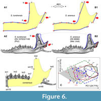Because the skull shape usually is not available in a fossil material, it was necessary to find differences in the shape of the hemimandible, especially because we knew that the two species differ well in the upper tooth row proportions (Appendix 5: Figure A5-1). PCA based on the hemimandible dataset on recent samples of S. araneus and S. tundrensis revealed a broad overlap between convex hulls of the two species; only SeV did not overlap with the S. tundrensis convex hull, whereas only a part of the S. tundrensis sample was separated (Figure 5B). Despite the similarity of the hemimandible shape, we detected the same transformation trends that we earlier found in the skull shape: (a) posterior shifting of the lower cheek-tooth row of S. tundrensis in relation to the short rostrum (Figure 6: A1 cf. Appendix 5: Figure A5-1); (b) an anterior shift of the mandibular ramus of S. tundrensis (an anterior tilt of the coronoid process, in particular) together with (c) an anterior shift of the condylar process in relation to the long braincase. These transformations were revealed at the negative end of the component; at the positive end of the component, we revealed the opposite shape transformation, specific for S. araneus (Figure 6: A2). Nevertheless, the broad similarity of the shape makes it impossible to separate the species and the description of the specific characteristics.

It is widely accepted that the size component plays a substantial role in species diversification. Usually, S. tundrensis is smaller in the overall size and certain linear measurements than S. araneus is. Some studies (Zaitsev, 1992, 1998; Fadeeva, 2016) point to the importance of the following mandibular characteristics in the species diagnostics: alveolar length of the lower molar row (aLML) and mandibular ramus height (MRH). We evaluated these characteristics within our mandibular dataset by normality tests and regression analysis (the von Bertalanffy model and linear model).

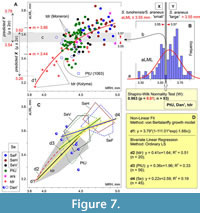The normality test uncovered a gap within the PtU/Dan'/ S. tundrensis combined sample in terms of the aLML parameter (Shapiro-Wilk W = 0.963, p < 0.01; n = 93; Figure 7). The gap covers a narrow interval between 3.55 and 3.57 mm and conventionally separates two groups: S. tundrensis/S. araneus “small” vs. S. araneus “large.” The regression analysis (von Bertalanffy model) regarding aLML vs. MHR showed a bend of the regression line in the overlap between S. tundrensis and PtU/Dan' (Figure 7A). We used the gap between size groups for calculation of predicted means and confidence intervals (μ ± 2σ, ca. 95% of the variance) of aLML. This procedure revealed the predicted overlap of two size groups in a broader interval between 3.54 and 3.62 mm (Figure 7A: c), whereas the observed overlap between “true” S. tundrensis and S. araneus in our analysis filled even broader intervals: between 3.33 and 3.64 mm in terms of aLML (0.31 mm) and between 4.25 and 4.61 mm in terms of MRH (0.36 mm). It should be noted that specimens of S. tundrensis from Moneron Island (an isolated population of S. tundrensis parvicaudatus Okhotina, 1976, in the Southern Okhotsk Sea) showed the longest aLML; the smallest values of aLML and MRH were displayed by S. tundrensis from the Kolyma River (ZIN 90453).

We tried to separately describe both parts of the bent von Bertalanffy model line (line d1, Figure 7A-C) using bivariate linear regression (the ordinary LS model). We calculated regression for three groups: (d2) S. tundrensis, (d3) the PtU sample, and (d4) combined Serov samples. A higher correlation and more pronounced aLML/MHR affine changes were shown by the S. tundrensis sample (R² = 0.51 [correlation value calculated with a permutation: 10,000 replicas; Hammer et al., 2001]; slope 0.41); slightly similar results with a weaker relationship were yielded by the PtU sample (R² = 0.33; slope 0.36). Both lines formed a lower part of the von Bertalanffy model line, approximately before the bend (Figure 7C: d2 and d3). The regression line of the Serov samples manifested the lowest correlation and the weak affine changes (R² = 0.19), when the aLML changes occur during weaker changes of MRH (lowest slope 0.22). Therefore, the regression analyses revealed an important pattern of the hemimandible shape variation that is true at least for the species studied here, namely: the mandibular shape similarity is due to the overall size, where small-sized specimens, regardless of species attribution, have a S. tundrensis -like shape morphotype (or something like that).

Morphospace Dynamics

In the current paper context, morphospace dynamics denote shape changes along certain trajectories of analyzed species in two respects: (i) changes of recent samples, e.g., between northern and southern localities; or (ii) changes of the fossil samples, e.g., between “Cold” and “Warm” intervals of the late Quaternary period. For the recent samples of S. araneus, we revealed a trajectory of changes of m1 and mandibular shapes in the direction of the S. tundrensis -like shape as size decreases from more southern (Serov) to more northern (Ulashevo) samples. The trajectory is more pronounced for the molar shape (Figure 5A) than mandibular shape (Figure 5B). In addition, the Serov subsamples showed similarity regardless of differences in altitude of habitats (a.s.l.; see the overlapping of Serov convex hull in Figure 5A).

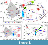For assessing temporal dynamics, we combined m1 datasets of recent and fossil samples, where we hypothesized some directions of the shape changes from DKS3 (10557 ± 234 cal BP, the Early Holocene), Cher1 (5673 ± 94 cal BP, the Middle Holocene), and Sim3/2a samples (2940 ± 258 cal BP, the Late Holocene; Figure 2, Appendix 2) to the recent samples. The PCAs revealed a similarity of the samples’ relationships that are shown in Figure 5A, except for an outlier of one fossil from Sim3 (S18), which contrary to our expectations, ended up at the negative end of PC1 (PtU/ S. tundrensis area; Figure 8A). For clear estimation of the relative position of the fossil teeth, we generated two separate insets for the S. tundrensis (Figure 8: B1) and S. araneus (Figure 8: B2) morphospace parts. In the insets, we can see a dense group of S. tundrensis from DKS3 (DK08-10; n = 3) outside the S. tundrensis convex hull but within the Dan' sample convex hull. Two specimens of S. araneus from Sim3 (except for the third one, S18) and their specimens from Cher1 lay within S. araneus convex hulls.

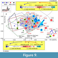Much more complex relationships between specimens and samples were found in mandibular morphospace (Figure 9A). Because the mandibular dataset was richer in fossil specimens (10 fossil m1/28 hemimandibles), we revealed at least two pronounced patterns, which was made possible only by the inclusion of the fossils: (i) there, a more complicated shape of the hemimandible was found in the S. tundrensis overall sample, which means the expansion of species morphospace due to the fossils. All fossil specimens of S. tundrensis from DKS3 proved to be outside S. araneus convex hulls (Serov/PtU); besides, two specimens from Sim3 (S18, similarly to m1 morphospace, and S19) lay far outside the S. tundrensis convex hull at the positive end of PC1 (Figure 9A); (ii) the centroid of the fossil samples of S. araneus, Sim3 (red squares), and DKS3 (blue squares) was unseparated, and both samples manifested a similarity to the S. tundrensis shape. For the interpretation of these differences that were shown by shape change trajectories, we estimated size differences between some samples (Table 3). The comparison results uncovered morphospace dynamics between the Early Holocene DKS3 sample, Late Holocene Sim3 sample, and recent sample (e.g., Dan') for both species.

First, the revealed trajectory of S. tundrensis describes unique proportion changes between Early Holocene DKS3 and Late Holocene Sim3 samples, where a notable size increase was associated with a shape shift outward from the recent species morphospace area, i.e., aLML values of S18 and S19 (μ = 3.66 mm) approached the S. araneus value (which is significantly greater than maximal aLML of S. tundrensis, Table 3), while the shape shifted to a new area. In the temporal interval between the Subboreal period of the Holocene (“Warm”; Sim3) to recent times (colder climate; Dan'), we revealed a size decrease that was associated with convergence of the mandibular shape between S. tundrensis and S. araneus (overlapping Dan' and PtU convex hulls, Figure 5B). Inset “B” in Figure 9 diagrammatically depicts this trajectory of the temporal changes of proportions (size + shape).

Second, the revealed trajectory of S. araneus describes almost absence of shape changes with time in relation to the S. tundrensis changes, i.e., between DKS3 and Sim3, the size increase was not accompanied by shape changes (Table 4: aLML cf. PC1, mean). On the other hand, the Dan' sample and the Middle Holocene sample from locality Cher1 showed a shape similarity together with size differences (means of aLML were 3.52 and 3.64, respectively). Therefore, for S. araneus, we observed inconsistency between temporal variations of size and shape. Mandibular morphospace manifested a shape shift between two groups of the sample: large S. araneus from the fossil sites, DKS3, and Sim3 vs. small-to-large S. araneus from the fossil site, Cher1, together with Dan'. The shape within each group varies insignificantly. Additionally, the first fossil group shared a shape similarity with recent S. tundrensis along with congruent size changes, whereas the second group approached the shapes of S. araneus recent samples. Inset “C” in Figure 9 diagrammatically illustrates the absence of a shape shift between DKS3 and Sim3 and a shift to the recent morphotype of the mandibular shape associated with a size decrease, e.g., in the Sim3/Dan' pair.

DISCUSSION

General Remarks

The concept of morphological variety and temporal alteration of phenotypic features is mostly based on morphometric techniques. Morphometry along with multivariate statistics or without it has always been used for assessing morphometric variation and changes and displacement of specific features within recent and fossil taxa (Butler and Greenwood, 1979; Butler et al., 1989; Rácz and Demeter, 1998; Zaitsev, 1992, 1998; Zaitsev and Osipova, 2005; Dokuchaev et al., 1999, 2010; Zazhigin and Voyta, 2022; and many others). The most common way to interpret the temporal changes in species features is to reveal size changes, e.g., within Bergmann's rule or for its exception (Homolka, 1980; Spitzenberger, 1980; Ochocińska and Taylor, 2003). We have known that environmental fluctuations can determine changes in shrew size, usually in contradiction to Bergmann’s rule, when cooling causes a size decrease and vice versa (Carraway and Verts, 2005; Rychlik et al., 2006; Panasenko and Kholin, 2011; Omelko and Kholin, 2017).

The independent estimation of environmental fluctuations in the past is made possible by faunal composition, abundance, and other parameters. In this case, we should have an intelligible initial hypothesis about how phenotypic alterations are consistent with faunal changes. The simplest hypothesis is a direct interaction between the phenotype and faunal composition during environmental changes (Brown and Wilson, 1956; Yom-Tov, 1991). Nevertheless, according to published studies, this is true for East Asian late Quaternary localities (Panasenko and Kholin, 2011; Omelko and Kholin, 2017), where we can see more or less consistent changes in shrew size and species abundance, especially for endemic species (e.g., S. mirabilis), and not true for Uralian late Quaternary localities (Zaitsev, 1992, 1998; Fadeeva, 2016), although those authors detected notable alterations of the faunal composition. For example, Zaitsev described a shift of S. tundrensis abundance from a predominant state (41.7%) in Early Holocene localities to a scarce state (few occurrences) in Late Holocene localities (Zaitsev, 1998: 154, 156). Contrary to expectations, Zaitsev (1992) for the Sim3 locality and Fadeeva (2016) for Pre-Uralian localities stated a similarity between fossil and recent samples of S. araneus and S. tundrensis. By contrast, Zaitsev (1998) supposed at least two new Sorex forms, Sorex sp. nov. 1 and Sorex sp. nov. 2, which “in mandibular size and proportions <...> are close to the group S. tundrensis ” (Zaitsev, 1998: 154). Furthermore, Fadeeva introduced a “forest form” of S. tundrensis and stated that the fossil remains from Pre-Uralian localities “are close to those of the modern tundra species of Russia’s European North” and “this form is characterized by a smaller size compared to the forest form” (Fadeeva, 2016: 168). The forest form of S. tundrensis was described by Bobretsov et al. (2008). The main features of the form are larger size than that shown by a nominative form and size similarity with S. araneus. In support of the broader size variation within the tundra shrew than we think, Yudin (1989: 249)–when describing dimensional variation of S. tundrensis by means of 684 specimens–gave a lower mean value of MRH than we can see in Bobretsov et al. (2008) and our study (Table 3): Yudin’s MRH = 4.20 ± 0.01 mm (μ ± SE) vs. Bobretsov’s MRH = 4.48 ± 0.02 mm (Dan') vs. our MRH = 4.42 mm (Dan'). Nonetheless, we can assume that Yudin’s overall sample of S. tundrensis specimens surely included the forest form because the range of limits significantly exceed the observed maximum MRH values (Yudin's limits = 3.08-4.80 mm) and even retrospectively includes the largest fossil remains of this species from Sim3 (S18 and S19; Table 3).

Perhaps the most important finding in the current paper is the presence of temporal morphospace dynamics revealed primarily for the mandibular shape of both S. araneus and S. tundrensis. This statement means that some fossil samples of both species have not been similar to recent samples. First, we noticed a frightening resemblance in m1 and mandibular datasets between recent samples of S. araneus and S. tundrensis from Russian-Plain localities PtU and Dan'. This resemblance is supported by Bobretsov et al. (2008), who already found this pattern precisely for Jani Peak, Garevka, and Dan' localities (Appendix 1: No. 2, 6, and 7).

Second, within the recent samples, we detected two opposite trajectories of shape changes: (i) a size decrease of S. araneus specimens associated with an increase of a shape similarity to S. tundrensis in both m1 and mandibular datasets, more pronounced in the latter dataset (Figure 5), and an opposite (ii) size increase of S. tundrensis specimens associated with a similarity to S. araneus. Accordingly, we found the part of morphospace where the two species considerably overlapped in shape, while having obvious differences in the skull shape (Appendix 5: Figure 5A-1) and linear dimensions (Bobretsov et al., 2008: 847). Intrinsic features of the mandibular shape convergence were partly detected by the regression analyses (Figure 7), where we see a difference in slope of the regression lines between large-sized S. araneus (line d4) and grouped small-sized S. araneus/S. tundrensis (line d3). These differences in slope mean a similarity in mandibular proportions (size + shape) within small-sized specimens regardless of species attribution.

Third, combining the recent and fossil samples within common morphospace revealed even more complex trajectories of the shape changes: (iii) within the S. tundrensis overall sample, there was a twofold shift in size and shape features from the Early Holocene DKS3 sample to the Late Holocene Sim3 and recent Dan' sample (Figure 9B). In size and shape, S. tundrensis from the DKS3 sample is closely related to the modern species sample (Appendix 1: T1-T5). This statement supports Fadeeva’s (2016) observation of a similarity between modern and fossil samples; (iv) a slightly warmer period of the Late Holocene (in comparison to the modern climatic conditions) formed the most distinguishable mandibular shape and the largest size of the fossil specimens from the Sim3 locality, which were different in shape both from the S. tundrensis overall sample and from the recent and fossil specimens of S. araneus (Figure 9). Of note, the size increase between DKS3 and Sim3 is followed by unexpected shape changes in the opposite direction of the modern trajectory (see point “ii” above); (v) however, a similar (to S. tundrensis) size increase between DKS3 and Sim3 samples of S. araneus did not cause significant shape changes (Table 4; Figure 9C), although we detected a clear shift in shape outside recent samples of S. araneus but within the recent sample of S. tundrensis. Overall, the aforementioned statements can be combined into the following conclusion: mandibular shape morphospace dynamics included at least an increase in morphological variety (disparity) of S. tundrensis from the Early Holocene (DKS3) to the Late Holocene (Sim3) and a more modest increase in the variety of S. araneus relative to the shape shifts in the fossil samples (DKS3 + Sim3). Therefore, the shape analyses together with the size data allowed us to reveal morphological changes, the causes of which are to be revealed in further studies involving richer fossil material.

Applicability of MEr, Shape, and Size Analyses

Most taxonomic and morphological investigations of recent and fossil data are based on morphometric approaches. Therefore, an assessment of MEr is becoming important, especially in paleontological data, due to the still modest suitability of the molecular approach and rare data mostly of small sample size. Sometimes, in published papers, we see high inconsistency of linear measurements of some type specimens that exceed differences between separate species, for example, dimensions of fossil type specimens of Beremendia pohaiensis (Kowalski and Li, 1963), holotype IVPP V2671, published in three studies, including the first description (Kowalski and Li, 1963). Each article provides holotype dimensions that differ from each other within a broad range, from 0.16 to 0.35 mm (Appendix 4: Figure A4-2), whereas differences between two species, e.g., B. pohaiensis vs. B. jiangnanensis Jin, Zhang, Sun and Zheng, 2009, are 0.25 mm (in mean values of Lm1 and Lm2; see Jin and Kawamura, 1996; Jin et al., 2009; Zazhigin and Voyta, 2019). Holotype dimensions of Beremendia pliocaenica Flynn et Wu, 1994 (IVPP V8900) published in the original description (Flynn and Wu, 1994) and a separate study (Jin and Kawamura, 1996) also showed inconsistency, which was 0.24 mm (Appendix 4: Figure A4-2).

In our analysis, we used three linear measurements, Lm1, aLML, and MRH, which are applied instead of the “centroid size” feature that is automatically produced during the Procrustes Fit procedure (Rohlf and Slice, 1990). For details on feature substitution, see the Methods section.

Among the main tasks, we used a linear dimension of m1 (lingual Lm1) for assessing ranges between a very precise measure by 3D models of m1 in the Avizo software (accuracy 6.0-7.3 mm) and a moderately precise measure by 2D images in the tpsDig2 digitizer (accuracy 0.01 mm), with a subsequent comparison of ranges with the observed dimensions of S. araneus and S. tundrensis. Results of the comparison indicated that 2D- and 3D-based measurements differ in the range of 0-0.06 mm in mean values and 0-0.14 mm in limits (Appendix 4: Table A4-11). The ranges between the two methods of measurement are less than differences between typical S. araneus (SeV) and S. tundrensis (samples T1-T7). Therefore, measurements using tpsDig2 will be accurate for further use together with calculation of the mean between three replicates.

Since geometric morphometric approaches (Rohlf and Slice, 1990; Zelditch et al., 2004; Claude, 2008; Adams, 2014; Schlager, 2017; and others) enable a more detailed analysis of morphological variations than linear dimensions, in this article, we applied geometric morphometry as the main method of morphological variety description. The first lower molar of shrews, just as other mammalian tribosphenic teeth, has a complex shape. Application of the geometric morphometric approaches to the analysis of such a tooth requires resolving the MEr issue. In the current study, we tried to estimate MEr of specimens’ orientation that arises during the acquisition of 2D occlusal shape of m1.

The result of application of the original MSMEr approach revealed a high proportion of MEr, which explained ~50% of the total variance within PC1-4 morphospace (Table 1). Subsequent variance components analysis revealed three components of the total variance along factors “Sample,” “Replicate,” and “Interception.” This technique indicated combined loading of MEr via factor “Replicate” (of 19.24%) and “Interception” (of 16.05%), with a specific loading of the “Sample” factor of 28.84% (Table 2). The second method of MEr estimation seems more accurate and gives more detailed results than the MSMEr approach does. Nonetheless, MSMEr gave an approximately similar estimate of the “Sample” factor and could visualize relationships between samples and replicates (Figure 4), which can be useful for quickly assessing the impact of MEr.

From two analyses, we can conclude that MEr has a significant impact on results and should be considered. On the other hand, the procedure of “analyses on the basis of mean values” has existed for a long time and minimizes the effects of MEr (e.g., “five times <...> m1” by Polly, 2003: 236). The data in Table 2 suggest that the analysis of mean values can reduce the effect of MEr and accordingly increase the significance of the original differences between samples.

Size/shape and Morphospace Dynamics

An increase in the complexity of morphospace was revealed after the addition of fossils (Figure 5, Figure 8, Figure 9). The complexity supports the thesis about the necessity of combined datasets consisting of fossil and recent samples of sympatric/coexisting species, in contrast to single-species analyses of recent samples (e.g., Voyta et al., 2013; Shchipanov et al., 2014; and others). Nevertheless, many aspects of temporal variation cannot be examined without prior testing of the recent data. In this context, a study of Rychlik et al. (2006) is considerably interesting. Those authors analyzed two sympatric species of water shrews, Neomys fodiens (Pennant, 1771) and N. anomalus Cabrera, 1907, using recent data in two aspects: the impact of environmental factors and the competition factor in size-shape variety. They documented four patterns of morphological variety that we attempted to use for the interpretation of our results, namely, (a) three morphological structures (skull, hemimandible, and m1) show different responses to environmental factors depending on different covariance patterns of each structure; (b) in sympatric samples, a smaller species manifests broader variation than large species do, which is explained by a subordinate position of the small species or probably by specificity of the analyzed samples to a small geographic area; (c) similarity of the m1 shape that is based on a similarity of diet; (d) “ecophenotypic plasticity”: a similarity increase for the sympatric samples as compared to allopatric one that, according to those authors, is based on a “similar ecophenotypic response to geoclimatic factors” and is also found, except for Neomys species, in S. araneus and S. coronatus sympatric samples (Rychlik et al., 2006: 348).

Two species, S. araneus and S. tundrensis, occur in the sympatric samples, e.g., in the South, Middle, and North Urals (SeF and SeH) and in Russian-Plain habitats (SeV, PtU, and Dan') (Bolshakov et al., 1996; Bobretsov et al., 2008; Bobretsov, 2016). These species are also found in the same layers of Upper Quaternary cave deposits from the South, Middle, and North Urals and Perm Pre-Ural (Zaitsev, 1992, 1998; Fadeeva, 2016). Unlike Rychlik et al. (2006), we did not initially regard sympatry as an important factor of the phenotypic variation; therefore, only one sympatric sample was present among the recent datasets: the Dan' sample. Unfortunately, the sample size did not permit us to check thesis “b” (see above), but we propose it as a major topic for further research and as a possible test for sympatry in fossil samples.

The subsamples from Dan' that corresponded to S. araneus and S. tundrensis showed a broad overlap both in size and shape in terms of m1 and mandibular datasets (Figure 5). We could correctly determine species attribution in Dan' only using the skull shape (Appendix 5: Figure A5-1). The specific feature of the Dan' sample is the smallest size of S. araneus and moderately large size of S. tundrensis (Table 3), which constitute this sample.

As reported for Neomys species (Rychlik et al., 2006), the biggest similarity between S. araneus and S. tundrensis was revealed in the molar shape (Figure 5). The m1 morphospace features almost a full overlap between PtU and S. tundrensis convex hulls (Figure 5A), whereas they only partly overlap within the mandibular morphospace (Figure 5B). Nonetheless, this result seems to depend on the landmark set and specific features of the species. Previously, for East Asian shrews, we demonstrated (Voyta et al., 2023) that the m1 shape can reveal two groups of the sympatric shrew: first, specialized species that ended up at the periphery of the morphospace (S. minutissimus, S. daphaenodon, S. caecutiens, and S. mirabilis), and second, “generalized” species that ended up at the center of the morphospace (S. araneus, S. isodon, and S. unguiculatus). In the present work, we seem to deal with species that are in the “generalized” group without obvious m1 shape differences. According to thesis “c” by Rychlik et al. (see above), a similarity in the m1 shape can be related first to a similarity of diet. Nevertheless, a more likely interpretation may involve a similarity of morphogenetic pathways within a sibling species. Because both species constitute the “araneus” species group (Bannikova et al., 2018), the m1 similarity can be explained in the morphogenetic context (Jernvall, 1995; Polly, 2005; Rychlik et al., 2006: 348; Kavanagh et al., 2007; Polly and Mock, 2018; Polly and Wójcik, 2019).

Another important statement by Rychlik et al. (2006) is more pronounced similarity within the sympatric samples, also supported by our results, at least for Dan'. The subsamples have undoubtedly coexisted and showed shape similarity in m1 and mandibular datasets. In the fossil samples, we can assess the species similarity in terms of coexistence only in the Early Holocene DKS3 sample with more than five specimens of each species (Appendix 2). This sample did not exhibit the patterns of the Dan' sample (Figure 9) because both species were found to be separated by size (aLML without overlapping of the limits) and shape (Table 4). This result could mean both the allopatry of subsamples (mixed fossil remains) and other responses/features of the species. Any of these features seems to have determined clear-cut size separation between the subsamples of DKS3. This is the key point of the difference between DKS3 and Dan' (except for time, of course). This topic surely merits further investigation.

Resolving Power of Tooth Shape

Despite the differences in the landmark sets between the current analysis and the paper by Voyta et al. (2023) cited above, we can say that there is a similar effect of the relatively “simple” landmark frame, which describes only crown shape but not the molar base. Hence, we lose a lot of information, despite the use of 3D data instead of 2D data. In the context of mammalian molar morphogenesis and its ecophenotypic component (Kavanagh et al., 2007; Polly and Mock, 2018; Polly and Wójcik, 2019), one can hypothesize an increase in resolving power of m1 shape with the increasing complexity of the landmark frame (e.g., Voyta et al., 2022a). A new landmark frame requires a transition to 3D datasets that involves proliferation of technical issues, including age-related effects (see Voyta et al., 2023: 579), and a lot processing time expended. In the current paper, we used 3D models, albeit in the simplest way: by replacing the taking of photos under a microscope, as Shchipanov et al. (2014) did, with capturing 2D images from 3D models. This approach was necessary to solve the MEr problem and is not mandatory otherwise. Nevertheless, in the context of our study, we seem to have been able to prove that the 2D m1 shape dataset can resolve many specific questions of variation description. Resolving power may be restricted only by certain features of species based on, e.g., phylogenetic affinity or trophic specialization. This conclusion allows us to regard 2D datasets as the most accessible and relatively powerful approach to geometric morphometric analysis of data collections through investigation of variation of both size and shape, not only size.

Our results of the m1 shape analysis revealed a significant similarity between small-sized S. araneus and S. tundrensis (Figure 5A); this similarity did not let us describe clear-cut differences among species. Therefore, we used two modern approaches that are based on 3D datasets and application of special packages from the R-statistics environment, phylomorphospace approach by Adams (2014) and 3D visualization of the paired comparison of shapes (Schlager, 2017; Appendix 6).

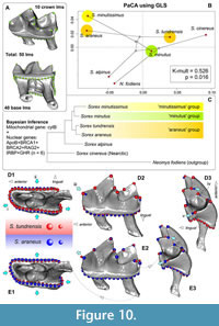We used the phylomorphospace of Adams (2014), which, except for the main purpose of “phylogenetic signal” assessment (Hulme-Beaman et al., 2019; Terray et al., 2022; Voet at al., 2022), also shows shape interactions against the background of existing trophic niches along phylogenetic affinities, i.e., we can see morphological diversification within clades simultaneously with ecophenotypic plasticity. If we complicate the landmark frame, e.g., go from seven to 50 landmarks, then we get visible differences between S. araneus and S. tundrensis in the m1 shape (Figure 10). The tooth of S. araneus differs from the S. tundrensis tooth by a wider and slightly shorter base of m1, a more posterior position of the paraconid tip, a deeper protocristid notch, and a longer hypolophid. Overall, some differences (paraconid shifting and the notch depth) were displayed by the 2D dataset (Figure 4).

The phylomorphospace based on a concatenated phylogenetic tree of seven soricine species gives a result slightly different from what we obtained here earlier (Figure 5A), namely, S. araneus is clearly separated from S. tundrensis. The two species–despite close phylogenetic affinity–ended up in different parts of space (Figure 10B). We observed a strong ecophenotypic plasticity effect and hence a relatively weak phylogenetic signal (K-mult = 0.526, p = 0.016; cf. Hulme-Beaman et al., 2019; Terray et al., 2022; Voet at al., 2022). The signal magnitude undoubtedly depends on the number of species and the landmark set (Blomberg et al., 2003); nevertheless, we achieved the specific purpose of using this approach, i.e., support for the following idea: a more complex landmark set can more precisely describe the m1 shape. It should not be forgotten, however, that the choice of the approach should be based on objectives of a given study and specifity of the purpose object; i.e., the complexity structure of a morphological element (e.g., skull as whole) includes several ‘morphogenetic modules’ (for shrew molars, e.g., in sense to Polly and Mock, 2018), therefore, an underestimation of the modules covariance can be lead to increased uncertainty. This uncertainty, in turn, can devalue any landmark set, even large 3D set, and seemly can provide a low phylogenetic signal (see Voet et al., 2022).

CONCLUSIONS

Several patterns were revealed in our study on morphological variety of S. araneus and S. tundrensis in the temporal aspect. Modern samples of both species show underestimated similarity both in size and in shape of morphological structures. Regression analysis detected different phenotypic traits of the mandibular proportion between large-sized and small-sized shrews regardless of species attribution. The size decrease of S. araneus and, conversely, a size increase of S. tundrensis, both drive the mandibular shape to sameness, i.e., represent phenotypic convergence. This pattern, however, is violated in the fossil samples, when the largest S. tundrensis from the Late Holocene Sim3 locality showed a well distinguishable mandibular shape in a separate part of the morphospace. Although in this case, morphospace capacity was enlarged by the addition of fossil species, there is a new issue: why did S. tundrensis show a new trajectory of shape changes at the Late Holocene locality? It seems likely that the differences in the traits between fossil and recent samples can be referred to as sympatry or allopatry in the sense of Rychlik et al. (2006); however, this topic will require further precise research in the context of “specialized” and “generalized” species, which we revealed by means of the m1 shape in East Asian shrews (Voyta et al., 2023). This context also involves an issue of resolving power of the morphological structures. In this study, we found that the m1 shape has week power in comparison to mandibular or especially skull shape. Nevertheless, even the moderate resolving power of the mandibular shape allowed us to reveal the phenotypic changes–during the Holocene–that have not been detected by previous researchers at Uralian late Quaternary localities. The most important conclusion from our results is the need to use modern approaches both in linear morphometry in combination with multivariate statistics and in geometric morphometry for analyses of multispecies datasets.

Prospects. The evidence outlined above suggests that environmental adaptation (or phenotypic plasticity) may be expressed in phenotypic convergence and has alternative ways of evolving. The presence of different trajectories of a proportion alteration in spatial and temporal aspects may determine a global direction of further investigations into recent and paleo communities within the framework of two hypotheses: “species collective response” by Clements (Lyons et al., 2010; DeSantis et al., 2012; Cooper et al., 2015; Kirchhoff, 2020) and “species-specific responses” by Gleason (Grayson, 2007; Lorenzen et al., 2011; Graham, 2014; Crees et al., 2016; Palombo, 2018) about global and regional climate changes in the sense of Puzachenko et al. (2022: 97). On the other hand, if two hypotheses of community responses help to reveal their adjusted strategies, then Shchipanov’s “hypothesis of functional structuring” (HFS) of small-mammal populations–with respect to a dependence of species diversity on the environmental diversity-disturbance relationship (Shchipanov, 2016)–may help to reveal specific strategies of community elements.

ACKNOWLEDGEMENTS

This study was funded by Project no. 22-24-00510 of the Russian Scientific Foundation. The study partly used the collection materials of the Zoological Institute of the Russian Academy of Sciences (St. Petersburg; http://www.ckp-rf.ru/usu/73561/) and Institute of Plant and Animal Ecology of Ural Branch of the Russian Academy of Sciences (Yekaterinburg). Authors are grateful to Dr. N.E. Dokuchaev for fulfill help in the S. tundrensis species identification in the Komi materials and particular information about East Asian Sorex data. Authors would like to thank Dr. A. Yu. Puzachenko for constructive discussion of MEr estimation, and Dr. F.V. Konstantinov for support our phylomorphospace analysis in the phylogenetic part (Appendix 6). Authors also are grateful to Prof. P.D. Polly and anonymous reviewer who refereed our manuscript and contributing to its improvement.

REFERENCES

Adams, D.C. 2014. Generalized K statistic for estimating phylogenetic signal from shape and other high-dimensional multivariate data. Systematic Biology, 63:685-697.
https://doi.org/10.1093/sysbio/syu030

Adler, D. and Murdoch, D. 2021. Package ‘rgl’, Version 0.104.16. Available at:
https://cran.r-project.org/web/packages/rgl/rgl.pdf

Agadjanian, A.K. 2009. Pliocene-Pleistocene small mammals of the Russian Plain. Nauka, Moscow. (In Russian)

Agustí, J. 1999. A critical re-evaluation of the Miocene mammal units in Western Europe: dispersal events and problems of correlation, p. 84-112. In Agustí, J., Rook, L., and Andrews P. (eds.), The evolution of Neogene terrestrial ecosystem in Europe. Cambridge University Press, New York.
https://doi.org/10.1017/cbo9780511542329.005

Andermann, T., Faurby, S., Turvey, S.T., Antonelly, A., and Silvesto, D. 2020. The past and future human impact on mammalian diversity. Science Advances, 6:eabb2313.
https://doi.org/10.1126/sciadv.abb2313

Andersen, K.K., Svensson, A., Johnsen, S.J., Rasmussen, S.O., Bigler, M., Röthlisberger, R., and Dahl-Jensen, D. 2006. The Greenland Ice Core chronology 2005, 15-42ka. Part 1: constructing the time scale. Quaternary Science Reviews, 25:3246-3257.
https://doi.org/10.1016/j.quascirev.2006.08.002

Baca, M., Nadachowski, A., Lipecki, G., Mackiewicz, P., Marciszak, A., Popović, D., Socha, P., Stefaniak, K., and Wojtal, P. 2017. Impact of climatic changes in the Late Pleistocene on migrations and extinctions of mammals in Europe: four case studies. Geological Quarterly, 61:291e304.
https://doi.org/10.1101/090878

Baca, M., Popović, D., Baca, K., Lemanik, A., Doan, K., Hotáček, López-García, J.M., Bañuls-Cardona, S., Pazonyi, P., Desclaux, E., Crégut-Bonnoure, E., Berto, C., Lenardić, J.M., Miękina, B., Murelaga, X., Cuenca-Bescós, G., Krajcarz, M., Marković, Z., Petculescu, A., Wilczyński, J., Knul, M.V., Stewart, J.R., and Nadachowski, A. 2020. Diverse responses of common vole (Microtus arvalis) populations to Late Glacial and Early Holocene climate changes e Evidence from ancient DNA. Quaternary Science Reviews, 233:10239.
https://doi.org/10.1016/j.quascirev.2020.106239

Banaszek, A., Smakulska, J., Fedyk, S., Jadwiszczak, K. A., and Chętnicki, W. 2003. Morphometric differentiation of shrews (Sorex araneus L., 1758) from hybrid zone between the Guzowy Młyn and Łęgucki Młyn chromosome races in Poland. Mammalia, 68:217-224.
https://doi.org/10.1515/mamm.2003.67.2.217

Bannikova, A.A., Chernetskaya, D., Raspopova A., Alexandrov, D., Fang, Y., Dokuchaev, N., Sheftel, B., and Lebedev, V. 2018. Evolutionary history of the genus Sorex (Soricidae, Eulipotyphla) as inferred from multigene data. Zoologica Scripta, 47:518-538.
https://doi.org/10.1111/zsc.12302

Bartlett, J.W. and Frost, C. 2008. Reliability, repeatability and reproducibility: analysis of measurement errors in continuous variables. Ultrasound in Obstetrics & Gynecology, 31:466-475.
https://doi.org/10.1002/uog.5256

Blomberg, S.P., Garland, T. Jr., and Ives, A.R. 2003. Testing for phylogenetic signal in comparative data: Behavioral traits are more labile. Evolution, 57:717-745.
https://doi.org/10.1554/0014-3820(2003)057[0717:tfpsic]2.0.co;2

Bobretsov A.V. 2016. Populatsionnaya ekologiya melkikh mlekopitayushchikh ravninnikh i gornikh landshaftov Severo-Vostoka evropeiskoi chasti Rossii. Izdatelstvo KMK, Moscow. (In Russian)

Bobretsov, A., Kupriyanova, I., Petrov, A., Demidova, T., and Shchipanov, N. 2008. A European forest form of Sorex tundrensis (Insectivora). Zoologicheskiy Zhurnal, 87:841-849 (In Russian, with English summary)

Bolshakov, V.N., Vasil'ev, A.G., and Sharova, L.P. 1996. Fauna i populatsionnaya ekologiya zemleroek Urala (Mammalia, Soricidae). Izdatelstvo “Ekaterinburg”, Ekaterinburg. (In Russian)

Bond, G.C. and Lotti, R. 1995. Iceberg discharges into the North Atlantic on millennial time scales during the Last Glaciation. Science, 267(5200):1005-1010.
https://doi.org/10.1126/science.267.5200.1005

Bookstein, F.L. 1991. Morphometric tools for landmark data: Geometry and Biology. Cambridge University Press, New York.
https://doi.org/10.1017/cbo9780511573064

Brown, W.L., Jr. and Wilson, E.O. 1956. Character displacement. Systematic Zoology, 5:49-64.
https://doi.org/10.2307/2411924

Bulatova, N.S., Biltueva, L.S., Pavlova S.V., Zhdanova N.S., and Zima, J. 2019. Chromosomal differentiation in the common shrew and related species, p. 134-185. In Searle, J.B., Zima, J., and Polly, P.D. (eds.), Shrews, Chromosomes and Speciation. Cambridge University Press, Cambridge.
https://doi.org/10.1017/9780511895531.006

Burgin, C.J. and He, K. 2018. Family Soricidae, p. 332-551. In Wilson, D.E. and Russell, A.M (eds.), Handbook of the mammals of the world. Vol. 8. Insectivores, sloths and colugos. Lynx Edicions, Barcelona.

Butler, P.M. and Greenwood, M. 1979. Soricidae (Mammalia) from the Early Pleistocene of Olduvai Gorge, Tansania. Zoological Journal of the Linnean Society, 67:329-379.
https://doi.org/10.1111/j.1096-3642.1979.tb01119.x

Butler, P.M., Thorpe, R.S., and Greenwood, M. 1989. Interspecific relations of African crocidurine shrews (Mammalia: Soricidae) based on multivariate analysis of mandibular data. Zoological Journal of the Linnean Society, 96:373-412.
https://doi.org/10.1111/j.1096-3642.1989.tb02520.x

Carraway, L.N. and Verts, B.J. 2005. Assessment of variation in cranial and mandibular dimensions in geographic races of Sorex trowbridgii, p. 139-153. In Merritt, J.F., Churchfield, S., Hutterer, R., and Sheftel, B.I. (eds.), Advances in the biology of shrews II. International Society of Shrew Biologists, New York.

Chętnicki, W., Fedyk, S., Banaszek, A., Szalaj, K.A., and Ratkiewicz, M. 1996. Morphometrical characteristics of the common shrew (Sorex araneus L.) from interracial hybrid zones. Hereditas, 125:201-207.
https://doi.org/10.1111/j.1601-5223.1996.00201.x

Churchfield, S. 1994. Foraging strategies of shrews, and the evidence from field studies, p. 77-88. In Merritt, J.F., Kirkland, G.L., Jr., and Rose, R.K. (eds.), Advances in the biology of Shrews. Carnegie Museum of Natural History, Pittsburg.

Claude, J. 2008. Morphometrics with R. Springer Science+Business Media, LLC, New York.

Cohen, K.M. and Gibbard, P.L. 2019. Global chronostratigraphical correlation table for the last 2.7 million years, version 2019 QI-500. Quaternary International, 500:20-31.
https://doi.org/10.1016/j.quaint.2019.03.009

Cooper, A., Turney, C., Hughen, K.A., Brook, B.W., McDonald, H.G., and Bradshaw, C.J.A. 2015. Abrupt warming events drove Late Pleistocene Holarctic megafaunal turnover. Science 349:602-606.
https://doi.org/10.1126/science.aac4315

Cornette, R., Baylac, M., Souter, T., and Herrel, A. 2013. Does shape co-variation between the skull and the mandible have functional consequences? A 3D approach for a 3D problem. Journal of Anatomy, 223:329-336.
https://doi.org/10.1111/joa.12086

Cornette, R., Tresset, A., and Herrel, A. 2015a. The shrew tamed by Wolff’s Law: Do functional constraints shape the skull through muscle and bone covariation? Journal of Morphology, 276:301-309.
https://doi.org/10.1002/jmor.20339

Cornette, R., Tresset, A., Houssin, C., Pascal, M., and Herrel, A. 2015b. Does bite force provide a competitive advantage in shrews? The case of the greater white-toothed shrew. Biological Journal of the Linnean Society, 114:795-807.
https://doi.org/10.1111/bij.12423

Crees, J.J., Carbone, C., Sommer, R.S., Benecke, N., and Turvey, S.T. 2016. Millennial-scale faunal record reveals differential resilience of European large mammals to human impacts across the Holocene. Proceedings of the Royal Society B: Biological Sciences, 283:20152152.
https://doi.org/10.1098/rspb.2015.2152

Daxner-Höck, G., Badamgarav, D., Erbajeva, M.A., and Göhlich, U. 2013. Miocene Mammal Biostratigraphy of Central Mongolia (Valley of Lakes): New Results, p. 477-494. In Wang, X., Flynn, L.J., and Fortelius, M. (eds.), Neogene Terrestrial Mammalian Biostratigraphy and Chronology of Asia. Columbia University Press, New York.
https://doi.org/10.7312/wang15012-020

deMenocal, P., Ortiz, J., Guilderson, T., Adkins, J., Sarnthein, M., Baker, L., and Yarusinsky, M. 2000. Abrupt onset and termination of the African Humid Period: rapid climate responses to gradual insolation forcing. Quaternary Science Reviews, 19:347-361.
https://doi.org/10.1016/s0277-3791(99)00081-5

DeSantis, L.R.G., Tracy, R.A., Koontz, C.S., Roseberry, J.C., and Velasco, M.C. 2012. Mammalian niche conservation through deep time. PLoS One 7:e35624.
https://doi.org/10.1371/journal.pone.0035624

Dokuchaev, N.E., Ohdachi, S., and Abe, H. 1999. Morphometric status of shrews of the Sorex caecutiens/shinto group in Japan. Mammal Study, 24:67-78.
https://doi.org/10.3106/mammalstudy.24.67

Dokuchaev, N.E., Kohno, N., and Ohdachi, S. 2010. Reexamination of fossil shrews (Sorex spp.) from the Middle Pleistocene of Honshu Island, Japan. Mammal Study, 35:157-168.
https://doi.org/10.3106/041.035.0302

Dudu, A., Churchfield, S., and Hutterer, R. 2005. Community structure and food niche relationships of coexisting rainforest shrews in the Masako Forest, Northeastern Congo, p. 229-239. In Merritt, J.F., Churchfield, S., Hutterer, R., and Sheftel, B.I. (eds.), Advances in the biology of shrews II. International Society of Shrew Biologists, New York.

Eble, G.J. 2000. Contrasting evolutionary flexibility in sister groups: disparity and diversity in Mesozoic atelostomate echinoids. Paleobiology, 26:56-79.
https://doi.org/10.1666/0094-8373(2000)026%3C0056:cefisg%3E2.0.co;2

Fadeeva, T. 2016. Insectivorous mammals (Lipotyphla, Soricidae) of the Perm Pre-Ural in the Late Pleistocene and Holocene time. Quaternary International, 420:156-170.
https://doi.org/10.1016/j.quaint.2015.10.074

Fadeeva, T.V. and Smirnov, N.G. 2008. Small Mammals of the Perm Pre-Urals in the Late Pleistocene and Holocene Time. Publishing House “Goshchitskii,” Yekaterinburg. (In Russian)

Flynn, L.J. and Wu, W. 1994. Two new shrews from the Pliocene of Yushe Vasin, Shanxi Province, China. Vertebrata PalAsiatica, 32:73-86.

Furió, M. and Agusti, J. 2017. Latest Miocene insectivores from Eastern Spain: Evidence for enhanced latitudinal differences during the Messinian. Geobios, 50:123-140.
https://doi.org/10.1016/j.geobios.2017.02.001

Furió, M., Santos-Cubedo, A., Minwer-Barakat, R., and Agusti, J. 2007. Evolutionary history of the African soricid Myosorex (Insectivora, Mammalia) out of Africa. Journal of Vertebrate Paleontology, 27:1018-1032.
https://doi.org/10.1671/0272-4634(2007)27[1018:ehotas]2.0.co;2

Furió, M., van ben Hoek Ostende, L.W., Agusti, J., and Minwer-Barakat, R. 2018. Evolution of the insectivore assemblages (Eulipotyphla, Mammalia) in Spain and their relation with Neogene and Quaternary climate changes. Ecosistemas, 27:38-51.
https://doi.org/10.7818/ecos.1454

Graham, R.W. 2014. Response of mammalian communities to environmental changes during the late Quaternary, p. 300-313. In Smith, F.A., Gittleman, J.L., and Brown, J.H. (eds.), Foundations of Macroecology. Classic Papers with Commentaries. University of Chicago Press, Chicago.

Grayson, D.K. 2007. Deciphering North American Pleistocene extinctions. Journal of Anthropological Research, 63:185-213.
https://doi.org/10.3998/jar.0521004.0063.205

Hammer, Ø., Harper, D.A.T., and Ryan, P.D. 2001. PAST: paleontological statistics soft-ware package for and data analysis. Palaeontologia Electronica, 4:1-9. Available from:
https://palaeo-electronica.org/2001_1/past/issue1_01.htm (accessed 03 April 2023)

Hanski, I. 1994. Population biological consequences of body size in Sorex, p. 15-26. In Merritt, J.F., Kirkland, G.L., Jr., and Rose, R.K. (eds.), Advances in the biology of Shrews. Carnegie Museum of Natural History, Pittsburg.

Happold, M. and Happold, D.C.D. 2013. Mammals of Africa: Hedgehogs, Shrews and Bats (Vol. IV). Bloomsbery Publishing, London.
https://doi.org/10.5040/9781472926944.0390

Homolka, M. 1980. Biometrischer vergleich zweier populationen Sorex araneus. Acta scientiarum naturalium Academiae Scientiarum Bohemicae, Brno, 14:1-34.

Hulme-Beaman, A., Claude, J., Chaval, Y., Evin, A., Morand, S., Vigne, J.D., Dobney, K., and Cucchi, T. 2019. Dental shape variation and phylogenetic signal in the Rattini tribe species of mainland Southeast Asia. Journal of Mammalian Evolution, 26:435-446.
https://doi.org/10.1007/s10914-017-9423-8

Hutterer, R. and Kryštufek, B. 2016. Sorex araneus (errata version published in 2017). The IUCN Red List of Threatened Species 2016: e.T29661A115170489.
https://doi.org/10.2305/IUCN.UK.2016-3.RLTS.T29661A22315145.en

Izvarin, E.P., Ulitko, A.I., and Nekrasov, A.E. 2020. Palaeontological description of Nizhneirginsky Grotto Upper Holocene sediments (Ufa Plateau, Fore-Urals) with taphonomic and palaeoenvironmental remarks based on bird and small-mammal assemblages. Quaternary International, 546:160-169.
https://doi.org/10.1016/j.quaint.2019.11.043

Izvarin, E., Ulitko, A., Panina, S., Zazovskaya, E., and Nekrasov, A. 2022. Voronin Grotto (Middle Urals, Russia): Analysis of vertebrate assemblage with taphonomic remarks and reconstruction of the Late Bronze Age and Early Iron Age human environment in the east end of Europe based on small mammals. Quaternary International, 632:178-191.
https://doi.org/10.1016/j.quaint.2022.02.031

Jackson, D.A. 1993. Stopping rules in principal components analysis: a comparison of heuristical and statistical approaches. Ecology, 74:2204-2214.
https://doi.org/10.2307/1939574

Jackson, S.T. and Blois, J.L. 2015. Community ecology in a changing environment: Perspectives from the Quaternary. Proceedings of the National Academy of Sciences, 112:4915-4921.
https://doi.org/10.1073/pnas.1403664111

Jernvall, J. 1995. Mammalian molar cusp patterns: developmental mechanisms of diversity. Acta Zoologica Fennica, 198:1-61.

Jin, C-Z. and Kawamura, Y. 1996. The first reliable record of Beremendia (Insectivora, Mammalia) in East Asia and a revision of Peisorex Kowalski and Li, 1963. Transactions and Proceedings of the Palaeontological Society of Japan, 182:432-447.

Jin, C-Z., Zhang, Y-Q., Sun, C-K., and Zheng, L-T. 2009. First discovery of the large shrew, Beremendia (Insectivora, Soricidae), from the lower Pleistocene of South China and its paleoclimatic implications. Vertebrata PalAsiatica, 4:153-163.

Kavanagh, K.D., Evans, A.R., and Jernvall, J. 2007. Predicting evolutionary patterns of mammalian teeth from development. Nature, 449:427-432.
https://doi.org/10.1038/nature06153

Kirchhoff, T. 2020. The myth of Frederic Clements’s mutualistic organicism, or: on the necessity to distinguish different concepts of organicism. History and Philosophy of the Life Sciences, 42:24(2020).
https://doi.org/10.1007/s40656-020-00317-y

Klingenberg, C.P. 2011. MorphoJ: an integrated software package for geometric morphometrics. Molecular Ecology Resources, 11:353-357.
https://doi.org/10.1111/j.1755-0998.2010.02924.x

Kotthoff, U., Müller, U.C., Pross, J., Schmiedl, G., Lawson, I.T., van de Schootbrugge, B., and Schulz, H. 2008. Lateglacial and Holocene vegetation dynamics in the Aegean region: an integrated view based on pollen data from marine and terrestrial archives. The Holocene, 18: 1019-1032.
https://doi.org/10.1177/0959683608095573

Koufos, G.D. 2013. Neogene Mammal Biostratigraphy and Chronology of Greece, p. 595-625. In Wang, X., Flynn, L.J., and Fortelius, M. (eds.), Neogene Terrestrial Mammalian Biostratigraphy and Chronology of Asia. Culumbia University Press, New York.
https://doi.org/10.7312/columbia/9780231150125.003.0028

Kowalski, K. and Li, C-K. 1963. A new form of the Soricidae (Insectivora) from the Pleistocene of North China. Vertebrata PalAsiatica, 7:138-143.

Lisiecki, L.E. and Raymo, M.E. 2005. A Pliocene-Pleistocene stack of 57 globally distributed benthic δ¹⁸O records. Paleoceanography, 20:PA1003.
https://doi.org/10.1029/2004pa001071

Lopatin, A.V. 2006. Early Paleogene insectivore mammals of Asia and establishment of the major group of Insectivora. Paleontological Journal, 40:205-405.
https://doi.org/10.1134/s0031030106090012

Lorenzen, E.D., Nogués-Bravo, D., Orlando, L., Weinstock, J., Binladen, J., Marske, K.A., Ugan, A., Borregaard, M.K., Gilbert, M.T.P., Nielsen, R., Ho, S.Y.W., Goebel, T., Graf, K.E., Byers, D., Stenderup, J.T., Rasmussen, M., Campos, P.F., Leonard, J.A., Koepfli, K.P., Froese, D., Zazula, G., Stafford, T.W., Aaris-Sørensen, K., Batra, P., Haywood, A.M., Singarayer, J.S., Valdes, P.J., Boeskorov, G., Burns, J.A., Davydov, S.P., Haile, J., Jenkins, D.L., Kosintsev, P., Kuznetsova, T., Lai, X., Martin, L.D., McDonald, H.G., Mol, D., Meldgaard, M., Munch, K., Stephan, E., Sablin, M., Sommer, R.S., Sipko, T., Scott, E., Suchard, M.A., Tikhonov, A., Willerslev, R., Wayne, R.K., Cooper, A., Hofreiter, M., Sher, A., Shapiro, B., Rahbek, C., and Willerslev, E. 2011. Species-specific responses of Late Quaternary megafauna to climate and humans. Nature, 479:359-364.
https://doi.org/10.1038/nature10574

Lyons, S.K., Wagner, P.J., and Dzikiewicz, K. 2010. Ecological correlates of range shifts of Late Pleistocene mammals. Philosophical Transactions of the Royal Society B, 365:3681-3693.
https://doi.org/10.1098/rstb.2010.0263

Martin, R.A. and Kelly, T.S. 2023. Biostratigraphy and biochronology of late Cenozoic North American rodent assemblages. Palaeontologia Electronica, 26(2):a29.
https://doi.org/10.26879/1303

Mishta, A. 2007. Morphometric variation of the common shrew Sorex araneus in Ukraine in relation to geoclimatic factors and karyotype. Russian Journal of Theriology, 6:51-62.
https://doi.org/10.15298/rusjtheriol.06.1.09

Mishta, A. and Searle, J.B. 2019. Morphology and genetics of the common shrew: General features, p. 68-111. In Searle, J.B., Zima, J., and Polly, P.D. (eds.), Shrews, Chromosomes and Speciation. Cambridge University Press, Cambridge.
https://doi.org/10.1017/9780511895531.004

Moya-Costa, R., Cuenca-Bescós, G., and Rofes, J. 2023. The shrews (Soricidae, Mammalia) of the Early and Middle Pleistocene of Gran Dolina (Atapuerca, Spain): reassessing their paleontological record in the Iberian Peninsula. Quaternary Science Reviews, 309:108093.
https://doi.org/10.1016/j.quascirev.2023.108093

Ochocińska, D. and Taylor, J.R.E. 2003. Bergmann’s rule in shrews: geographical variation of body size in Palearctic Sorex species. Biological Journal of the Linnean Society, 78:365-381.
https://doi.org/10.1046/j.1095-8312.2003.00150.x

Omelko, V.E. and Kholin, S.K. 2017. Secular variability of brown-toothed shrews (Sorex, Eulipotyphla) from the Southern Sikhote-Alin in the Late Quaternary. Zoologicheskii Zhurnal, 96:222-231. (In Russian, with English summary)

Omelko, V.E., Kuzmin, Y.V., Tiunov, M.P., Voyta, L.L., and Burr, G.S. 2020. Late Pleistocene and Holocene small mammal (Lipotyphla, Rodentia, Lagomorpha) remains from Medvezhyi Klyk Cave in the Southern Russian Far East. Proceedings of the Zoological Institute RAS, 324:124-145.
https://doi.org/10.31610/trudyzin/2020.324.1.124

Palombo, M.R. 2018. Faunal dynamics in SW Europe during the late Early Pleistocene: Palaeobiogeographical insights and biochronological issues. Comptes Rendus Palevol, 17:247-261.
https://doi.org/10.1016/j.crpv.2017.09.003

Panasenko, V.E. and Kholin, S.K. 2011. Historical aspect of the lower jaw variability of Crocidura shantungensis Miller, 1901 (Eulipotyphla: Soricidae). Amurian Zoological Journal III(4):391-396.

Polly, P.D. 2003. Paleogeography of Sorex araneus (Insectivora, Soricidae): molar shape as a morphological marker for fossil shrews. Mammalia, 68:233-243.
https://doi.org/10.1515/mamm.2003.67.2.233

Polly, P.D. 2005. Development and phenotypic correlations: the evolution of tooth shape in Sorex araneus. Evolution & Development, 7:29-41.
https://doi.org/10.1111/j.1525-142x.2005.05004.x

Polly, P.D. 2007. Phylogeographic differentiation in Sorex araneus: Morphology in relation to geography and karyotype. Russian Journal of Theriology, 6:73-84.
https://doi.org/10.15298/rusjtheriol.06.1.11

Polly, P.D. 2019. Climate, diversification and refugia in the common shrew: Evidence from the fossil record, p. 407-454. In Searle, J.B., Zima, J., and Polly, P.D. (eds.), Shrews, Chromosomes and Speciation. Cambridge University Press, Cambridge.
https://doi.org/10.1017/9780511895531.014

Polly, P.D. 2023. Extinction and morphospace occupation: A critical review. Cambridge Prisms: Extinction, 1(e17):1-9.
https://doi.org/10.1017/ext.2023.16

Polly, P.D. and Mock, O.B. 2018. Heritability: the link between development and the microevolution of molar tooth form. Historical Biology, 30:53-63.
https://doi.org/10.1080/08912963.2017.1337760

Polly, P.D. and Wójcik, J.M. 2019. Geometric morphometric tests for phenotypic divergence between chromosomal races, p. 336-364. In Searle, J.B., Zima, J., and Polly, P.D. (eds.), Shrews, Chromosomes and Speciation. Cambridge University Press, Cambridge.
https://doi.org/10.1017/9780511895531.011

Polyakov, A.V., Onischenko, S.S., Ilyashenko, V.B., Searle, J.B., and Borodin, P.M. 2002. Morphometric difference between the Novosibirsk and Thomsk chromosome races of Sorex araneus in a zone of parapatry. Acta Theriologica, 47:381-387.
https://doi.org/10.1007/bf03192464

Ponomarev, D. and Andreicheva, L. 2019. Middle-Upper Quaternary stratigraphy in the northeast of European Russia inferred from rodent record and lithology of tills. Quaternary International, 534:60-72.
https://doi.org/10.1016/j.quaint.2018.11.025

Prins, J., McCormack, D., Michelson, D., Horrell K., and Tobias, P. 2012. Product and Process Comparisons (Chapter 7). In Croarkin. C. and Tobias, P. (eds.), NIST/SEMATECH e-Handbook of Statistical Methods.
https://doi.org/10.18434/M32189

Prost, S., Klietmann, J., van Kolfschoten, T., Guralnick, R.P., Waltari, E., Vrieling, K., Stiller, M., Nagel, D., Rabeder, G., Hofreiter, M., and Sommer, R.S. 2013. Effects of Late Quaternary climate change on Palearctic shrews. Global Change Biology, 19(6):1865-1874.
https://doi.org/10.1111/gcb.12153

Puzachenko, A.Yu., Markova, A.K., and Pawlowska, K. 2022. Evolution of Central European regional mammal assemblages between the late Middle Pleistocene and the Holocene (MIS7-MIS1). Quaternary International, 633:80-102.
https://doi.org/10.1016/j.quaint.2021.11.009

Rácz, G. and Demeter, A. 1998. Character displacement in mandible shape and size in two species of water shrews (Neomys, Mammalia: Insectivora). Acta Zoologica Academiae Scientiarum Hungaricae, 44:165-175.

Railsback, L.B., Gibbard. P.L., Head. M.J., Voarintsoa. N.R.G., and Toucanne. S. 2015. An optimized scheme of lettered marine isotope substages for the last 1.0 million years, and the climatostratigraphic nature of isotope stages and substages. Quaternary Science Reviews, 111:94-106.
https://doi.org/10.1016/j.quascirev.2015.01.012

Rasmussen, S.O., Andersen, K.K., Svensson, A.M., Steffensen, J.P., Vinthe,r B.M., Clausen, H.B., Siggaard-Andersen, M.-L., Johnsen, S.J., Larsen, L.B., Dahl-Jensen, D., Bigler, M., Röthlisberger, R., Fischer, H., Goto-Azuma, K., Hansson, M.E., and Ruth, U. 2006. A new Greenland ice core chronology for the last glacial termination. Journal of Geophysical Research: Atmospheres, 111:D06102.
https://doi.org/10.1029/2005jd006079

Rasmussen, S.O., Bigler, M., Blockley, S.P., Blunier, T., Buchardt, S.L., Clausen, H.B., Cvijanovic, I., Dahl-Jensen, D., Johnsen, S.J., Fischer, H., Gkinis, V., Guillevic, M., Hoek, W.Z., Lowe, J., Pedro, J.B., Popp, T., Seierstad, I.K., Steffensen, J.P., Svensson, A.M., Vallelonga, P., Vinther, B.M., Walker, M.J.C., and Winstrup, M. 2014. A stratigraphic framework for abrupt climatic changes during the Last Glacial period based on three synchronized Greenland ice-core records: refining and extending the INTIMATE event stratigraphy. Quaternary Science Reviews, 106:14-28.
https://doi.org/10.1016/j.quascirev.2014.09.007

Reimer, P.J., Austin, W.E.N., Bard, E., Bayliss, A., Blackwell, P.G., Ramsey, C.B., Butzin, M., Cheng, H., Edwards, R.L., Friedrich, M., Grootes, P.M., Guilderson, T.P., Hajdas, I., Heaton, T.J., Hogg, A,G., Hughen, K.A., Kromer, B., Manning, S.W., Muscheler, R., Palmer, J.G., Pearson, C., van der Plicht, J., Reimer, R.W., Richards, D.A., Scott, E.M., Southon, J.R., Turney, C.S.M., Wacker, L., Adolphi, F., Büntgen, U., Capano, M., Fahrni, S.M., Fogtmann-Schulz, A., Friedrich, R., Köhler, P., Kudsk, S., Miyake, F., Olsen, J., Reinig, F., Sakamoto, M., Sookdeo, A., and Talamo, S. 2020. The INTCAL20 Northern Hemisphere radiocarbon age calibration curve (0-55 cal kbp). Radiocarbon, 62:725-757.
https://doi.org/10.1017/rdc.2020.41

Reumer, J.W.F. 1984. Ruscinian and Early Pleistocene Soricidae (Insectivora, Mammalia) from Tegelen (The Netherlands) and Hungary. Scripta Geologica, 73:1-173.

Rofes, J., Cucchi, T., Hanot, P., Herman, J., Stephan, P., Cersoy, S., Horáček, I., Kerr, E., Allberry, K., Valenzuela, S., Zazzo, A., Cornette, R., and Tresset, A. 2018. Postglacial recolonization and Holocene diversification of Crocidura suaveolens (Mammalia, Soricidae) on the north-western fringe of the European continent. Quaternary Science Reviews, 190:1-10.
https://doi.org/10.1016/j.quascirev.2018.04.016

Rohlf, F.J. 2003. tpsRelw, version 1.35.
http://life.bio.sunysb.edu/morph/index.html (accessed January 2023)

Rohlf, F.J. 2004. tpsUtil, version 1.28.
http://life.bio.sunysb.edu/morph/index.html (accessed January 2023)

Rohlf, F.J. 2007. tpsDig2, version 2.31.
http://life.bio.sunysb.edu/morph/index.html (accessed January 2023)

Rohlf, F.G and Slice, D.E. 1990. Extension of the Procrustes method for the optimal superimposition of landmarks. Systematic Zoology, 39:40-59.
https://doi.org/10.2307/2992207

Rychlik, L., Ramalhinho, G., and Polly, P.D. 2006. Response to environmental factors and competition: skull, mandible and tooth shapes in Polish water shrews (Neomys, Soricidae, Mammalia). Journal of Zoology and Systematics, 44:339-351.
https://doi.org/10.1111/j.1439-0469.2006.00374.x

Rzebik-Kowalska, B. 1998. Fossil history of shrews in Europe, p. 23-92. In Wójcik, J.M. and Wolsan, M. (eds.), Evolution of Shrews. Mammal Research Institute Polish Academy of Sciences, Białowieża.

Rzebik-Kowalska, B. 2006. Erinaceomorpha and Soricomorpha (Mammalia) from the Late Pleistocene and Holocene of Krucza Skała Rock Shelter and Komorowa Cave (Poland). Acta Zoologica Cracoviensia, 49A:83‒118.
https://doi.org/10.3409/000000006783995481

Schlager, S. 2017. Morpho and Rvcg - Shape Analysis in R: R-packages for geometric morphometrics, shape analysis and surface manipulations, p. 217-256. In Zheng, G., Li, S., and Szekely, G. (eds.), Statistical Shape and Deformation Analysis, 1st. Edition. Academic Press Inc., San Diego.
https://doi.org/10.1016/b978-0-12-810493-4.00011-0

Searle, J.B. and Thorpe, R.S. 1987. Morphometric variation of the common shrew (Sorex araneus) in Britain, in relation to karyotype and geography. Journal of Zoology, 212:373-7.
https://doi.org/10.1111/j.1469-7998.1987.tb06003.x

Searle, J.B. and Wójcik, J.M. 1998. Chromosomal evolution: The case of Sorex araneus, p. 219-268. In Wójcik, J.M. and Wolsan, M. (eds.), Evolution of Shrews. Mammal Research Institute Polish Academy of Sciences, Białowieża.

Shchipanov, N.A., Voyta, L.L., Bobrtsov, A.V., and Kuprianova I.F. 2014. Intra-species structuring in the common shrew Sorex araneus (Lipotyphla: Soricidae) in European Russia: morphometric variability could give evidence of limitation of interpopulation migration. Russian Journal of Theriology, 13:119-140.
https://doi.org/10.15298/rusjtheriol.13.2.08

Smirnov, N.G. 1993. Small mammals of the Middle Urals in Late Pleistocene/Holocene. Nauka, Ekaterinburg. (In Russian)

Smirnov, N.G., Bolshakov, V.N., Kosintsev, P.A., Panova, N.K., Korobeinikov, Yu.I., Olshvang, V.N., Erokhin, N.G., and Bykova, G.V. 1990. Istoricheskaya ekologiya zhivotnikh gor Yuzhnogo Urala. UrO AN SSSR, Sverdlovsk.

Smirnov, N.G., Izvarin, E.P., Kuzmina, E.A., and Kropacheva, Y.E. 2016. Steppe species in the Late Pleistocene and Holocene small mammal community of the Urals. Quaternary International, 420:136-144.
https://doi.org/10.1016/j.quaint.2015.10.112

Spitzenberger, F. 1980. Sumpf-und Wasserspitzmaus (Neomys anomalus Cabera, 1907 und Neomys fodiens Pennant, 1771). Mitteilungen der Abteilung für Zoologie und Botanik am Landesmuseum Joanneum, Graz, 9:1-39.

Strukova, T.V., Bachura, O.P., Borodin, A.V., and Stefanovskii, V.V. 2006. Mammal fauna first found in alluvial-speleogenic formations of the Late Neopleistocene and Holocene, Northern Urals, locality Cheremukhovo-1. Stratigraphy and Geological Correlation, 14:91-101.
https://doi.org/10.1134/s0869593806010060

Svensson, A., Andersen, K., Bigler, M., Clausen, H.B., Dahl-Jensen, D., Davies, S.M., Johnsen, S.J., Muscheler, R., Parrenin, F., Rasmussen, S.O., Röthlisberger, R., Seierstad, I., Steffensen, J.P., and Vinther, B.M. 2008. A 60 000 year Greenland stratigraphic ice core chronology. Climate of the Past, 4:47-57.
https://doi.org/10.5194/cp-4-47-2008

Taylor, J.R.E., Muturi, M., Lázaro, J., Zub, K., and Dechmann, D.K.N. 2022. Fifty years of data show the effects of climate on overall skull size and the extent of seasonal reversible skull size changes (Dehnel’s phenomenon) in the common shrew. Ecology and Evolution, 12:e9447.
https://doi.org/10.22541/au.164321458.83547834/v1

Terray, L., Denys, C., Goodman, S.M., Soarimalala, V., Lalis, A., and Cornette, R. 2022. Skull morphological evolution in Malagasy endemic Nesomyinae rodents. PLoS ONE, 17:e026304.
https://doi.org/10.1371/journal.pone.0263045

Thaw, S., White, T.A., Bannikova, A.A., and Searle, J.B. 2019. Phylogeography, p. 112-133. In Searle, J.B., Zima, J., and Polly, P.D. (eds.), Shrews, Chromosomes and Speciation. Cambridge University Press, Cambridge.
https://doi.org/10.1017/9780511895531.005

Tsytsulina, K., Formozov, N., Sheftel, B., Stubbe, M., Samiya, R., Ariunbold, J., and Buuveibaatar, V. 2016. Sorex tundrensis (errata version published in 2017). The IUCN Red List of Threatened Species 2016: e.T41422A115185726.
https://doi.org/10.2305/IUCN.UK.2016-3.RLTS.T41422A22318424.en

Ulitko, A.I. 2006. Golotsenovye mlekopitaushchie iz karstovykh polostei Srednego Urala, p. 243-247. In Savinetcky A.B. (ed.), Dinamika sovremennykh ekosistem v golotsene. Materialy Rossiyskoy nauchnoy konferentsii. Izdatelstvo KMK, Moscow. (In Russian)

Van Dam, J.A. 2004. Anourosoricini (Mammalia: Soricidae) from the Mediterranean region: A pre-Quaternary example of recurrent climate-controlled north-south range shifting. Journal of Paleontology, 78:741-764.
https://doi.org/10.1666/0022-3360(2004)078%3C0741:amsftm%3E2.0.co;2

Viacava, P., Blomberg, S.P., and Weisbecker, V. 2023. The relative performance of geometric morphometrics and linear-based methods in the taxonomic resolution of a mammalian species complex. Ecology and Evolution, 13:e9698.
https://doi.org/10.22541/au.165573736.65712166/v1

Voet, I., Denys, C., Colyn, M., Lalis, A., Konečny, A., Dlapré, A., Nicolas, V., and Cornette, R. 2022. Incongruences between morphology and molecular phylogeny provide an insight into the diversification of the Crocidura poensis species complex. Scientific Reports, 12:e10531.
https://doi.org/10.1038/s41598-022-12615-5

Voyta, L.L., Omelko, V.E., and Petrova, E.A. 2013. Analysis of the morphometric variability and intraspecific structure of Sorex minutissimus Zimmermann, 1780 (Lipotyphla: Soricidae) in Russia. Proceedings of the Zoological Institute RAS, 317:332-351. (In Russian, with English summary)
https://doi.org/10.31610/trudyzin/2013.317.3.332

Voyta, L.L., Omelko, V.E., Tiunov, M.P., and Vinokurova, M.A. 2021. When beremendiin shrews disappeared in East Asia, or how we can estimate fossil redeposition. Historical Biology, 33:2656-2667.
https://doi.org/10.1080/08912963.2020.1822354

Voyta, L.L., Omelko, V.E., Tiunov, M.P., Petrova, E.A., and Kryuchkova, L.Yu. 2022a. Temporal variation in soricid dentition: which are first - qualitative or quantitative features? Historical Biology, 34:1901-1915.
https://doi.org/10.1080/08912963.2021.1986040

Voyta, L.L., Abramov, A.V., Lavrenchenko, L.A., Nicolas, V., Petrova, E.A., and Kryuchkova, L.Y. 2022b. Dental polymorphisms in Crocidura (Soricomorpha: Soricidae) and evolutionary diversification of crocidurine shrew dentition. Zoological Journal of the Linnean Society, 196:1069-1093.
https://doi.org/10.1093/zoolinnean/zlab103

Voyta, L.L., Omelko, V.E., Izvarin E.P., Kropacheva, Yu.E., Eidinova, E.O., Shemyakina, Yu.A., Nikiforova, V.S., Strukova, T.V., and Smirnov, N.G. 2023. Late Quaternary communities of shrews, Soricidae, from Ural and Far East Regions of Russia: A protocol for the multifactorial morphospace building. Proceedings of the Zoological Institute RAS, 327:555-590. (In Russian, with English summary)
https://doi.org/10.31610/trudyzin/2023.327.3.555

White, T.A., Wójcik, J.M., and Searle, J.B. 2019. Phylogenetic relationships of chromosomal races, p. 186-216. In Searle, J.B., Zima, J., and Polly, P.D. (eds.), Shrews, Chromosomes and Speciation. Cambridge University Press, Cambridge.
https://doi.org/10.1017/9780511895531.007

Willis, K.J., Bailey, R.M., Bhagwat, S.A., and Birks, H.J.B. 2010. Biodiversity baselines, thresholds and resilience: testing predictions and assumptions using palaeoecological data. Trends in Ecology and Evolution, 25:583-591.
https://doi.org/10.1016/j.tree.2010.07.006

Wills, M., Briggs, D.E.G., and Fortey, R.A. 1994. Disparity as an evolutionary index: a comparison of Cambrian and Recent arthropods. Paleobiology, 20:93-130.
https://doi.org/10.1017/s009483730001263x

Wójcik, J.M., Bogdanowicz, W., Pucek, Z., Wуjcik, A.M., and Zalewska, H. 2000. Morphometric variation of the common shrew Sorex araneus in Poland, in relation to karyotype. Acta Theriologica, 45:161-72.
https://doi.org/10.4098/at.arch.00-71

Wójcik, J.M., Wуjcik, A.M., and Sikorski, M.D. 2003. Morphometric variation in the common shrew, Sorex araneus, in different habitats. Mammalia, 68:225-31.
https://doi.org/10.1515/mamm.2003.67.2.225

Yom-Tov, Y. 1991. Character displacement in the psammophile Gerbillidae of Israel. Oikos, 60:173-179. https://doi.org/10.2307/3544863

Yudin, B.S. 1989. Insectivorous Mammals of Siberia. Nauka, Novosibirsk. (In Russian)

Zaitsev, M.V. 1992. Insectivorous mammals of the Late Antropogene of South Ural, p. 61-80. In Smirnov, N.G. (ed.), The history of modern fauna of South Ural. UrO RAN Press, Sverdlovsk. (In Russian)

Zaitsev, M.V. 1998. Late Anthropogene Insectivora from the South Urals with a special reference to diagnostics of red-toothed shrews of the genus Sorex, p. 145-158. In Saunders, J.J., Styles, B.W., and Baryshnikov G.F. (eds.), Quaternary Paieozoofogy in the Northern Hemispher. Illinois State Museum Scientific Papers, Vol. XXVII. Springfield.

Zaitsev, M.V. and Osipova, V.A. 2005. Insectivorous mammals (Insectivora) of the Late Pleistocene in the Northern Caucasus. Zoologicheskiy Zhurnal, 83:851-868. (In Russian, with English summary)

Zaitsev, M.V., Voyta, L.L., and Sheftel, B.I. 2014. The mammals of Russia and adjacent territories. Lipotyphlans. Nauka, St. Petersburg. (In Russian)

Zazhigin, V.S. and Voyta, L.L. 2018. A new middle Miocene crocidosoricine shrew from the Mongolian Shargain Gobi Desert. Acta Palaeontologica Polonica, 63:171-187.
https://doi.org/10.4202/app.00396.2017

Zazhigin, V.S. and Voyta, L.L. 2019. Northern Asian Pliocene-Pleistocene beremendiin shrews (Mammalia, Lipotyphla, Soricidae): a description of material from Russia (Siberia), Kazakhstan, and Mongolia and the paleobiology of Beremendia. Journal of Paleontology, 93:1234-1257.
https://doi.org/10.1017/jpa.2019.51

Zazhigin, V.S. and Voyta, L.L. 2022. New Neogene anourosoricin shrews from northern Asia. Palaeontologia Electronica, 25(3):a29.
https://doi.org/10.26879/1209

Zelditch, M.L., Swiderski, D.L., Sheets, H.D., and Fink, W.L. 2004. Geometric morphometrics for Biologists: A Primer. Elsevier Academic Press, London.
https://doi.org/10.1016/b978-0-12-778460-1.x5000-5

Zima, J. and Searle, J.B. 2019. Milestones in common shrew chromosomal research, p. 1-18. In Searle, J.B., Zima, J., and Polly, P.D. (eds.), Shrews, Chromosomes and Speciation. Cambridge University Press, Cambridge.
https://doi.org/10.1017/9780511895531.002