The starting shape and P matrix for the simulations were estimated from a sample of the European Common shrew, Sorex araneus, from Bialowieza National Forest, Poland (N = 43), housed in the Mammal Research Institute of the Polish Academy of Sciences at Bialowieza. The first molar of each individual was photographed through a microscope in functional occlusal view (Butler 1961; Crompton 1971), a position that is less prone to orientation error than other views (Polly 2001a, 2003a). Each specimen was photographed five times and averaged to minimize further the error due to orientation and landmark placement. 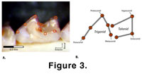Nine two-dimensional landmarks were placed on major crown cusps and notches to represent the morphology of the tooth (Figure 3) and superimposed using Procrustes (GLS) superimposition (Gower 1975; Rohlf 1999). In principle, this simulation could be carried out with 3-D representations of shape, but two dimensions were used here to facilitate comparison with existing data on variation in shrew molar morphology. The mean of the superimposed teeth was used as the starting morphology for each simulation.

P was estimated as the covariance matrix of the Procrustes residuals of the superimposed landmarks that remain after the mean shape is subtracted (Table 1). With nine two-dimensional landmarks, there were a total of 18 residual shape variables, making P an 18 x 18 matrix. P only has 15 non-zero eigenvectors, however, because three dimensions are lost due to the removal of variation in size, translation, and rotation during superimposition (Table 2). Each simulation, therefore, required a vector H with 15 elements, one for each dimension of the PC space.

The elements of H were randomly generated at each step of the simulation. Each simulation drew elements from a distribution appropriate to the mode of evolution being modelled, as described below. The median H for all of the simulations except genetic drift was based on the rate of evolution of molar shape in Cantius (Primates, Mammalia) from the early Eocene of Wyoming (Clyde and Gingerich 1994). These authors estimated the average per-generation rate of change in Bookstein shape coordinates using the log-rate/log-interval (LRI) method (Gingerich 1993). LRI rates are reported in units of phenotypic standard deviations per generation, or haldanes, which are equivalent to the square root of H. Gingerich and Clyde estimated a rate of 0.653 haldanes per landmark dimension, the squared value of which (0.426) was used as the standard deviation for most of the H distributions in this paper. The accuracy of this rate and its appropriateness for shrew molars are arguable, but it is the only empirical estimate of the rate of evolutionary change in molar shape that is available.

Effective population size, N_e, is the main parameter required for simulating genetic drift (Wright 1931). Drift occurs when population means differ from one generation to the next because some individuals fail to reproduce by chance: the smaller the population size, the greater the effect. The expected change due to drift is equal to the heritable morphological variance divided by N_e (Lande 1976). N_e is not easy to estimate in living animals because population sizes fluctuate over time. In practice, N_e is estimated either from population censuses or from molecular markers (Avise et al. 1988; Avise 1994, 2000); the latter usually produces much larger estimates because it represents an average over large geographic and temporal scales. The simulation of drift was run twice, once with N_e = 70, an estimate based on population censuses (Churchfield 1982, 1990, personal commun., 2004; Wójcik, personal commun., 2004), and once with N_e = 70,000, an estimate based on molecular estimates (Ratkiewiecz et al. 2002).

Each simulation required the random H elements to be generated in a different way. For the simulation of random selection, the elements were drawn from a normal distribution centred on zero with a standard deviation of 0.426. This distribution yields numbers that are equally likely to be positive or negative, with a mean absolute magnitude of 0.338. Directional coefficients were drawn from a skewed distribution, with the probability of a negative value marginally higher than a positive one, but still with an absolute magnitude of 0.338. A negative bias was arbitrarily applied to all eigenvectors, though directional selection would still obtain if the direction were positive in some dimensions and negative in others. Stabilizing selection had coefficients drawn from a normal distribution with a standard deviation of 0.426, but whose mean depended on the value of the phenotype. When the phenotype fell in the negative direction from the starting value on a particular axis, then the mean of the H was positive, thus tending to push the phenotype back towards its original form. Drift was simulated using a H distribution centred on zero with a standard deviation equal to each eigenvalue divided by N_e. Each of these distributions is explained in more detail with each simulation. Note that a different random coefficient was drawn for each dimension at each generation in all simulations. Also note that the same mode was applied to all eigenvectors in each simulation; in principle, one could apply drift to some dimensions, directional selection to others, and stabilizing selection to some in any combination. None of the simulations can be considered deterministic or to be based on a "constant" rate or direction of evolution because the coefficients were randomly selected from a range of values that changed direction and magnitude each generation.

Procrustes distance was used as a measure of divergence of shapes from the starting configuration. Procrustes distance is the square root of the sum of squared differences in the positions of the landmarks in two shapes (Slice et al. 1996; Dryden and Mardia 1998). Procrustes distance is a Mahalonobis distance that represents the overall difference in the phenotype. The same Procrustes distance can describe the difference between many landmark configurations (Rohlf and Slice 1990). Though disadvantageous in some contexts, this property is useful because the distribution of distances reveals some aspects of the mode of evolution.

Changes in the phenotype are illustrated in some animations as thin-plate spline (tps) deformation grids showing the difference between the evolved shape and the starting configuration. The grids were constructed using techniques described in Bookstein (1989).