RESULTS
Randomly fluctuating selection, in which the direction and intensity of selection changes at each generation, was modelled in the first simulation. This mode of evolution occurs when morphological fitness is influenced by many independent factors (e.g., mate choice, nutrition, winter temperature, predator density), each of which vacillates from year to year with changing environments and functional contexts. Randomly fluctuating selection is a type of random walk, or Brownian motion, because the direction and magnitude of change in any given generation is not influenced by that in earlier or later ones.
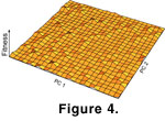 The randomly fluctuating mode is equivalent to evolution with a flat adaptive landscape, but one that has stochastic ripples in its surface
(Figure 4). The landscape is flat because there is no particular direction in which fitness increases, but its surface ripples because selection is constantly pushing the morphology in one direction or another. This mode is not an example of genetic drift or neutral evolution. In drift, the change between generations is due solely to chance and is purely a function of variance and population size, whereas the selection coefficients applied here were larger than expected from drift. A simulation of genetic drift would have an adaptive surface that is flat and still because selection would not affect the morphology at all (see below). See
Arnold et al. (2001) for a recent introduction to adaptive landscapes and multivariate evolution.
The randomly fluctuating mode is equivalent to evolution with a flat adaptive landscape, but one that has stochastic ripples in its surface
(Figure 4). The landscape is flat because there is no particular direction in which fitness increases, but its surface ripples because selection is constantly pushing the morphology in one direction or another. This mode is not an example of genetic drift or neutral evolution. In drift, the change between generations is due solely to chance and is purely a function of variance and population size, whereas the selection coefficients applied here were larger than expected from drift. A simulation of genetic drift would have an adaptive surface that is flat and still because selection would not affect the morphology at all (see below). See
Arnold et al. (2001) for a recent introduction to adaptive landscapes and multivariate evolution.
Selection coefficients for each of the 15 dimensions of the shape space were drawn each generation from a normal distribution with a mean of zero and a standard deviation of 0.426. These coefficients have an equal probability of being positive or negative and a mean absolute magnitude of 0.338. The simulation was run 100 times for 1,000,000 generations each run.
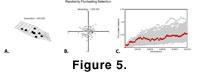 In the randomly varying mode of evolution, the 100 evolving shapes diffused randomly through the simulation space in an ever-enlarging cloud
(Figure 5). Even though the mean rate of evolution was lower than that measured in
Cantius, it was high enough so that in many of the runs the tooth shape evolved into functionally nonviable forms, as illustrated by the particular run shown in the left panel. A narrower distribution of selection coefficients (i.e., a smaller mean rate of per-generational change) would not have produced such extreme shapes.
The evolution of nonsense molar shapes suggests that the
P matrix is incompatible with a rate of evolution this high under this mode of selection, implying (1) that the
true rate of molar evolution in shrews is lower; (2) that true rate of evolution
is of a similar magnitude, but the
P matrix changes to accommodate this rate and still maintains a functional tooth; or (3) that stabilizing selection removes the nonviable morphologies in the course of real evolution.
In the randomly varying mode of evolution, the 100 evolving shapes diffused randomly through the simulation space in an ever-enlarging cloud
(Figure 5). Even though the mean rate of evolution was lower than that measured in
Cantius, it was high enough so that in many of the runs the tooth shape evolved into functionally nonviable forms, as illustrated by the particular run shown in the left panel. A narrower distribution of selection coefficients (i.e., a smaller mean rate of per-generational change) would not have produced such extreme shapes.
The evolution of nonsense molar shapes suggests that the
P matrix is incompatible with a rate of evolution this high under this mode of selection, implying (1) that the
true rate of molar evolution in shrews is lower; (2) that true rate of evolution
is of a similar magnitude, but the
P matrix changes to accommodate this rate and still maintains a functional tooth; or (3) that stabilizing selection removes the nonviable morphologies in the course of real evolution.
The most important result of this simulation is the distribution of morphological distances relative to the number of generations elapsed
(Figure 5C). Procrustes distance from the ancestral form increased curvilinearly as a function of the square root of the number of generations elapsed. As the simulation proceeded, larger divergences in shape became more probable, while the likelihood of no divergence decreased. Put another way, we may expect multivariate morphological shape to diverge from its ancestral condition in a curvilinear fashion under random fluctuating selection. This pattern has implications for reconstructing phylogeny from morphometric shape and for estimating divergence times based on morphological differences, as discussed below.
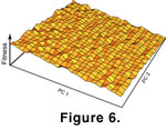 Directional selection, in which selection more often causes changes in one direction than another, was modelled in the second simulation. The preponderance of selection coefficients was in the negative direction, but with a stochastic component to both direction and magnitude at each generation. This mode of evolution is equivalent to an adaptive landscape that slopes ever upwards so that fitness is generally higher in the negative direction, but
with stochastic fluctuation creates short-lived, small scale increases in fitness in other directions
(Figure 6). The tilt of this landscape is determined by the degree of positive or negative bias in the selection coefficients, which was chosen arbitrarily for this simulation.
Directional selection, in which selection more often causes changes in one direction than another, was modelled in the second simulation. The preponderance of selection coefficients was in the negative direction, but with a stochastic component to both direction and magnitude at each generation. This mode of evolution is equivalent to an adaptive landscape that slopes ever upwards so that fitness is generally higher in the negative direction, but
with stochastic fluctuation creates short-lived, small scale increases in fitness in other directions
(Figure 6). The tilt of this landscape is determined by the degree of positive or negative bias in the selection coefficients, which was chosen arbitrarily for this simulation.
To carry out this simulation, selection coefficients were drawn from a Gamma distribution whose
 and
and  parameters were 100 and 0.1 respectively, scaled to have a mean of zero and a standard deviation of 0.426. A Gamma distribution is skewed in one direction or the other, and coefficients drawn from this one have the same mean intensity as in
Simulation 1, but 54% of them are negative. The simulation was run 100 times for 1,000,000 generations each run.
parameters were 100 and 0.1 respectively, scaled to have a mean of zero and a standard deviation of 0.426. A Gamma distribution is skewed in one direction or the other, and coefficients drawn from this one have the same mean intensity as in
Simulation 1, but 54% of them are negative. The simulation was run 100 times for 1,000,000 generations each run.
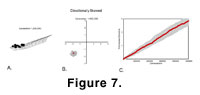 The results show a rapid rate of morphological change that is clearly directional whether viewed as a morphological reconstruction, as the cloud of points in phenotypic space, or the change in Procrustes distance with time
(Figure 7). Even though the average magnitude of selection at any given generation was the same as in the first simulation, the magnitude of morphological change over the entire simulation was more than six times higher as measured in Procrustes distances. The consistent changes in the same direction throughout the simulation cause this apparently rapid and dramatic change, whereas in the randomly fluctuating mode the morphology often doubled back in a homoplastic manner, making the greatest changes from the ancestral form much smaller. The rate of directional change depends on the proportion of negative to positive coefficients. Had the proportion of negative values been less than 54%, then the departure from the ancestral form would have been slower.
The results show a rapid rate of morphological change that is clearly directional whether viewed as a morphological reconstruction, as the cloud of points in phenotypic space, or the change in Procrustes distance with time
(Figure 7). Even though the average magnitude of selection at any given generation was the same as in the first simulation, the magnitude of morphological change over the entire simulation was more than six times higher as measured in Procrustes distances. The consistent changes in the same direction throughout the simulation cause this apparently rapid and dramatic change, whereas in the randomly fluctuating mode the morphology often doubled back in a homoplastic manner, making the greatest changes from the ancestral form much smaller. The rate of directional change depends on the proportion of negative to positive coefficients. Had the proportion of negative values been less than 54%, then the departure from the ancestral form would have been slower.
Stabilizing selection, in which selection pushes the morphology back towards the ancestral form if it moves too far away, was modelled in the third simulation. Stabilizing selection keeps a population at an optimum
(Schmalhausen
1949). The intensity of selection increases as the population mean moves away from the optimum, culling morphologies that are radically different. In palaeontology, stabilizing selection is one of several processes thought to explain patterns of morphological stasis
(Vrba and Eldredge 1984;
Maynard Smith et al. 1985;
Lieberman et al.
1995).
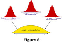 Stabilizing selection was simulated here using a single-peaked adaptive landscape to adjust the distribution from which selection coefficients were drawn
(Figure 8). The peak represents the optimal form, and the slopes represent morphologies that are less fit. Mathematically, the adaptive landscape surface and corresponding selection distributions are described by
Lande (1976) and
Arnold et al.
(2001).
Stabilizing selection was simulated here using a single-peaked adaptive landscape to adjust the distribution from which selection coefficients were drawn
(Figure 8). The peak represents the optimal form, and the slopes represent morphologies that are less fit. Mathematically, the adaptive landscape surface and corresponding selection distributions are described by
Lande (1976) and
Arnold et al.
(2001).
The adaptive surface is a Gaussian normal fitness curve whose width is 0.85 Procrustes units. When the simulated morphology is at the peak, selection coefficients are drawn from a normal distribution with a mean of zero and a standard deviation of 0.426, precisely the same distribution as in the simulation of randomly fluctuating selection. The width of the peak is about three times larger than the average magnitude of the selection coefficients when the morphology is at the peak (0.29 Procrustes units). Because of this small proportional difference, the stabilizing selection in this simulation is quite strong.
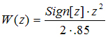
As the simulated morphology moves off the peak, the mean of the distribution of coefficients is shifted in an opposite direction so that the chance of a positive coefficient increased as the morphology moves in a negative direction and vice versa. Mathematically, the following fitness function was used
-
 , (3)
, (3)
 in which W(z) is the fitness of the phenotype at position
z on the peak. Position of zero is the top of the peak. This equation was translated into a modification of the selection coefficients by adding
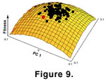
W(z) to the mean of the distribution from which they were drawn. Thus, when the morphology moves in a negative direction, the mean of the distribution increases and pushes the morphology back in a positive direction. The random nature of the distribution of coefficients adds a stochastic component to the direction and magnitude of selection
(Figure 9).
in which W(z) is the fitness of the phenotype at position
z on the peak. Position of zero is the top of the peak. This equation was translated into a modification of the selection coefficients by adding
W(z) to the mean of the distribution from which they were drawn. Thus, when the morphology moves in a negative direction, the mean of the distribution increases and pushes the morphology back in a positive direction. The random nature of the distribution of coefficients adds a stochastic component to the direction and magnitude of selection
(Figure 9).
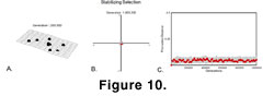 The results of this simulation showed a rapid morphological divergence from the mean during the first few thousand generations but one that quickly stabilized at a fixed mean from the ancestral form
(Figure 10). Stabilizing selection kept the morphology stable, and the diffusion through principal components space was small and concentrated. Most notably, the Procrustes distances of the 100 runs remained very small.
The results of this simulation showed a rapid morphological divergence from the mean during the first few thousand generations but one that quickly stabilized at a fixed mean from the ancestral form
(Figure 10). Stabilizing selection kept the morphology stable, and the diffusion through principal components space was small and concentrated. Most notably, the Procrustes distances of the 100 runs remained very small.
 Genetic drift, or random change in the population mean due to generational sampling in the absence of selection, was modelled in the fourth simulation. Like random selection, genetic drift is a type of random walk. The difference between drift and random selection is that the magnitude of change at each generation is much smaller in the former than the latter. In drift, the rate of per-generation change is a function of the phenotypic variance (literally the heritable variance) and population size
(Wright 1931;
Lande
1976). Drift is equivalent to evolution on a flat, placid adaptive landscape
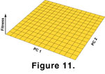
(Figure 11). The phenotype is neither more nor less fit, no matter which way it moves, and there is no stochastic selection to create transient ripples in the surface.
Genetic drift, or random change in the population mean due to generational sampling in the absence of selection, was modelled in the fourth simulation. Like random selection, genetic drift is a type of random walk. The difference between drift and random selection is that the magnitude of change at each generation is much smaller in the former than the latter. In drift, the rate of per-generation change is a function of the phenotypic variance (literally the heritable variance) and population size
(Wright 1931;
Lande
1976). Drift is equivalent to evolution on a flat, placid adaptive landscape
(Figure 11). The phenotype is neither more nor less fit, no matter which way it moves, and there is no stochastic selection to create transient ripples in the surface.
The amount of change in each generation depends only on the phenotypic variance and long-term effective population size (Ne), with change being smaller when the population is larger. I ran two simulations of drift because of the discrepancy between molecular and field estimates of population size in
Sorex araneus: one used Ne = 70,000 and the other Ne = 70.
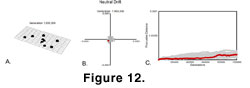 When Ne was 70,000, absolutely no change was visible in the phenotype at any time during the simulation
(Figure 12). The 100 runs diffused through the principal components space with the same pattern as in randomly fluctuating selection, but the average distance travelled was about five orders of magnitude smaller. When
Ne was dropped to 70, some phenotypic change was visible (Figure
13), but considerably less than under stabilizing selection.
When Ne was 70,000, absolutely no change was visible in the phenotype at any time during the simulation
(Figure 12). The 100 runs diffused through the principal components space with the same pattern as in randomly fluctuating selection, but the average distance travelled was about five orders of magnitude smaller. When
Ne was dropped to 70, some phenotypic change was visible (Figure
13), but considerably less than under stabilizing selection. 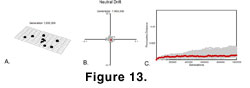 This result suggests that the amount of change in molar morphology due to drift is very, very small, even over 1,000,000 generations (roughly equivalent to 1,000,000 years).
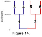 Randomly fluctuating selection with speciation was modelled in the final simulation. The mode of evolution in this simulation was the same as in the first, but instead of treating each run as a single evolving lineage, the lineage branched twice, once at the beginning of the simulation and then again halfway through
(Figure 14). Each simulation was run 100 times for 1,000,000 generations.
Randomly fluctuating selection with speciation was modelled in the final simulation. The mode of evolution in this simulation was the same as in the first, but instead of treating each run as a single evolving lineage, the lineage branched twice, once at the beginning of the simulation and then again halfway through
(Figure 14). Each simulation was run 100 times for 1,000,000 generations.
This simulation shows how derived morphological similarity accumulates within clades
(Figure 15). During the first 500,000 generations, the two stem lineages diverge randomly from one another, creating two derived ancestral morphologies for their respective daughter species.
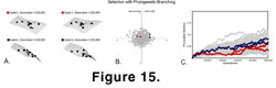 By the end of the simulation, those shared derived phenotypes are still visible, even though each terminal phenotype has its own autapomorphic condition. Shared phylogenetic
history also leaves its trace in the positions of the phenotypes within the PC space. The daughter species of the first clade (red dots) remained relatively close to one another but distant the daughters of the second (blue dots).
By the end of the simulation, those shared derived phenotypes are still visible, even though each terminal phenotype has its own autapomorphic condition. Shared phylogenetic
history also leaves its trace in the positions of the phenotypes within the PC space. The daughter species of the first clade (red dots) remained relatively close to one another but distant the daughters of the second (blue dots).
