ACCURACY OF MECHANICAL DIGITIZING DATA

Any 3D file is only of use if it mirrors the original object accurately enough for the investigation at hand. As described above there exists an inverse relationship between accuracy and file size. The smaller files produced from mechanical digitizing offer the benefit of easier handling over the large files from laser or CT scanning, but is their accuracy sufficient for e.g. skeletal reconstructions or rapid prototyping of scale models? In order to test this, a number of mechanical digitizing files were compared to the high-resolution CT based files scaled down to the same final size as the mechanical digitizing files. The following virtual bones of GPIT1 Plateosaurus engelhardti were used in order to cover different sizes and shapes: left humerus, left ilium, second dorsal vertebra. Additionally, the pedal phalanx II-1 from GPIT 2 Plateosaurus engelhardti was digitized. The files were imported into Geomagic® and aligned automatically with the 'Best fit' option. A 3D comparison analysis was performed, creating a 3D map of the surface pair, in which distance between the surfaces at any point is displayed by varying colors. The program also calculates the maximum, average, and standard deviations. Note that the actual errors of the mechanical digitizing files are probably smaller than determined by the program, because the alignment was not optimized for minimal deviation. Geomagic® offers a variety of alignment options, but we considered it unnecessary to test which one offers the smallest deviation values.

Ilium: The CT data of the left ilium consisted of 1778 slices, of which 889 (every second) were used to extract the file. The reduction was made necessary by the fact that each slice of 0.5 mm thickness overlapped the neighboring files by half that amount, which for unknown reasons created massive artifacts (wrinkling) in the finished surfaces. The scan of the ilium also included the right fibula, totaling a data volume of 894 MB at 516 kB per file. From it, an STL file in ASCII format with 203 MB was extracted. This file, which still included pieces of the fibula and internal 3D bodies in the ilium, was edited to gain the maximum resolution STL file of the ilium in Rhinoceros®, having shrunk to 47 MB by removal of the excess data and saving in binary STL format. One deep pit stemming from obvious damage was removed by manual editing. The file has 977244 triangles and was reduced in Geomagic® to 89816 (9,19%) to achieve the same file size as the point cloud file.

The point cloud data consisted initially of 44865 points, which were meshed into a surface with 89816 polygons. This was edited manually to remove some obvious artifacts along sharp edges, where curvature-based filling was applied. Also, various small artifacts on flat surfaces were removed. The files size is 4,33 MB.

For the 3D deviation comparison a display scale was selected that details deviations of between +/- 0.5 mm and +/- 5 mm. Deviations smaller than half a millimeter we assume to be irrelevant. Deviations up to 2.5 mm are tolerable, and for values up to 5 mm (~ 1% of greatest length of the ilium) it is important where they occur. If strong deviations are limited to damaged areas of the bone, they can be ignored outright. On the other hand, several millimeters of deviation over larger areas are unacceptable. Any deviation greater than half a centimeter can only be tolerated if it has no influence on the likely shape of the undamaged bones, i.e., if it occurs due to damage of the specimen. The likeliest scenario for such a deviation is a tiny, deep hole in the bone that must be passed over with the digitizer.

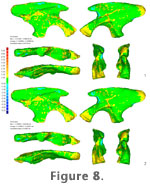Figure 8.1 shows the 3D deviation maps of the pointcloud based file compared to the CT file. Deviation ranges from nearly +5 mm to almost -15 mm, but values greater than 2.5 mm occur exclusively near cracks in the bone. The mechanical digitizing file preserves a different 3D body than the CT scan data in such places, because it is limited to gathering data at the air/solid boundary, while in the CT file some of the crack infill is missing, because the extraction threshold was set roughly at the bone/sediment boundary. Geomagic detects and ignores non-alignable areas, but the edges of these areas are assessed. Despite these, average deviation is below 0.5 mm.

To test how significant the influence of the shape differences caused by the cracks is, the CT based file was extensively edited to smooth the cracks over. This lead to the removal of further internal surfaces and created 43 holes in the outer surface, all of which were automatically closed by curvature-based filling. In all, the number of polygons dropped by 15.8% to 75658 polygons, reducing file size to 3,6 MB. 3D comparing this file to the point cloud file (Figure 8.2) resulted in a significant reduction of the maximum deviations (+4.12 mm / -3.1 mm). The average and standard deviations were little influenced, in contrast, due to the large undamaged surface areas, which outweigh the cracks.

Humerus: The humerus based on NURBS curves, created in roughly seven minutes, was lofted in Rhinoceros® with a loft rebuild option with 25 control points, and exported for comparison in Geomagic® as a polymesh file with 13764 polygons. The original NURBS file has a size of 1.27 MB.

The mechanical digitizing file with points consisted of 24640 points, with only a handful of obviously erroneous points. Digitizing time was roughly 10 minutes. Meshing in Geomagic® produced a surface with various small and two large holes. All could be filled with curvature-based filling without problems. The file was now manually smoothed, after which 49102 polygons remained. Figure 4 shows the original point cloud, the wrapped surface, and the edited final surface. The file size is 2.47 MB, nearly double that of the NURBS file.

The CT data of the left humerus stemmed from an earlier scanning opportunity and had a lower resolution than all later CT scans. The STL file extracted from 282 MB of raw data initially had a size of 359.202 MB (ASCII STL) and 1763876 polygons. It was reduced to 2.81% to match the 49524 polygons of the point cloud file. This operation alone required over 12 minutes calculation time on a 2.4 GHz PC with 2 GB of RAM and a 256MB graphics card.

Figure 9 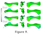shows the 3D deviation maps for the pointcloud (Figure 9.1) and NURBS (Figure 9.2) files using the same scale as the ilium comparisons (+/- 0.5 mm to +/- 5 mm). Average deviation is ~ 0.2 mm for the point clouds file and ~0.4 mm for the NURBS file. In contrast, maximum deviation is significantly different between the two files. While the point clouds file differs at most 1.61 mm in one small location on the humeral crest, the NURBS file shows larger areas of strong deviation along prominent edges. The extreme value of over 15 mm, however, is limited to a small spot, where apparently a lofting artifact creates a deep indentation in the loft file. Note that the large holes in the original mesh (Figure 4.2) do not result in large errors in the final surface due to the use of the curvature-based filling algorithm.

Pedal Phalanx II-1: The point cloud file, created in roughly four minutes, consisted of 9212 points after removal of erroneous points. The mesh created from it required some editing due to internal polygons. They were apparently caused by small errors during recalibrations, leading to a suboptimal fit between the point clouds created before and after recalibrations. The file size is 906 kB with 18540 polygons after smoothing. The NURBS file, a rebuild loft with 100 control points, was created in 10 minutes, most of which was spent taping and marking the bone. It has a size of 933 kb as a STL.

The left pedal phalanx II-1 was CT scanned along with various other small elements. Original size was 170054 polygons and 33.1 MB. After surface extraction, it was reduced to 18540 polygons (10.9%) as well.

Because of the much smaller size of the phalanx compared to the ilium (roughly 18% if maximum lengths are compared), it appears unreasonable to demand the same degree of absolute accuracy for digital files of both. Acceptable error should be expressed not as an absolute value (e.g., 2.5 mm), but as a percentage of total size (e.g., 2.5% of largest dimension). Therefore, the phalanx files were 3D compared using two different scales: the same scale that was used for the ilium and humerus (0 – +/- 5 mm deviation, with the minimum displayed deviation greater than +/- 0.5 mm), and a scale with one fifth the values: 0 – +/- 1mm, minimum displayed > +/- 0.1 mm.

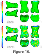
The NURBS file 3D deviation maps for both scales are given in Figure 10. Although the average deviation is very small at ~ 0.1 mm, maximum deviations of slightly over 2.5 mm occur at the sharp dorsal edge of the proximal articulation surface and on the medial distal condyle. However, these are three localized deviations that do not appear to alter the general shape of the edge if the 5 mm scale is used to assess the differences (Figure 10.1). Using the tighter 1 mm scale, in contrast, exposes deviations of 0.5% maximum specimen length along all edges (Figure 10.2) and shows that this deviation is continuous along the dorsal margin and the distal condyle. This means that the compound error when measuring across these two points may exceed 1% of maximum length.

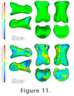
The point cloud file deviations are shown in Figure 11.1 (5 mm scale) and Figure 11.2 (1 mm scale). Here, average deviation is more than double that of the NURBS file, and the errors are widely spread over the bone surfaces. Maximum deviation, though, is much lower, expect for one artifact on the ventral side near the proximal end.

Dorsal 2: The CT data, which had the same wrinkling problems as the ilium file, was reduced to 28266 triangles for use in the virtual skeleton. It shall serve here as an example of an object with a complex shape combined with a small file size. The mechanical digitizing file, with 51582 points (41592 after removal of obviously erroneous points), was meshed in Geomagic® and required some filling of holes. It took nearly 12 minutes to create. Spikes were removed on an average setting. Now the file contained 8611 polygons. It was now reduced to 28266 polygons (32.83%), to fit the CT based file. The size is now 1.381 MB. 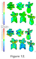Figure 12 shows the 3D deviation, both using the 5 mm scale (Figure 12.1) and a size adjusted scale running from +/- 0.125 mm to +/- 1.25 mm (Figure 12.2). The standard deviation at less than 0.4 mm is tolerable, but many edges show strong deviation along their entire lengths. The maximum deviation of over 7 mm occurs along the sharp edges of the left postzygapophysis. These deviations indicate that the problem rests with the meshing of the point cloud in places where interpoint distances are similar between points on the same surface and points on different surfaces (upper and lower face of the zygapophysal process). Note that the point cloud file has an artificially constructed neural canal, while the canal of the fossil is filled with matrix. High deviations in this area are to be expected and meaningless for digitizing accuracy.

In general, the 3D deviation analyses show that – at the file size of mechanical digitizing with point clouds or NURBS curves – the accuracy of both CT and mechanical digitizing data is sufficiently similar to allow using the various formats interchangeably for most applications. At the maximum resolution of CT data available to us, the deviations are probably marginally larger. However, comparing the reduced CT files of all four bones to the maximum sized ones in 3D deviation analyses resulted in differences only in places where

there were extremely fine cracks,
there were very fine connections between internal and external surfaces (irrelevant for mechanical digitizing), or
there were 'wrinkling' artifacts present in the high-resolution surface, apparently caused by the overlap of neighboring slices.

These differences all remained under 0.1% of the greatest length of the bone. Therefore, the reduced CT files can serve as an accurate model of the high-resolution files.

Our sample number is low, but except for very large bones or extremely thin structures (e.g., sauropod vertebral laminae) all typical problems are represented by the sample. Generally, it is possible to mechanically digitize mid-sized to large bones (>20 cm greatest length) with errors below 0.5% of the maximum length or 1 mm. While one of the files we used to assess the accuracy of our methods, the dorsal 2 file, is close to this size class and shows significantly higher errors, it is important to note that this point cloud file was our first attempt at digitizing a vertebra at all. The deviations, spread out over nearly all the surface, and consistently positive or negative over relatively wide areas of the bone, are apparently caused by insufficiently accurate calibration of the digitizer between the different point cloud parts. The complex shape of the specimen and our inexperience in mechanical digitizing lead to a high number of recalibrations, along with the instable support of the specimen in a sandbox. The deviations evident in Figure 12.2 underscore the importance of both stable support for the specimen and as few recalibrations as possible during the digitizing process. Files smaller than 20 cm maximum length are probably better digitized using point clouds.

There is no general pattern of one of the two mechanical digitizing methods being more accurate or faster. NURBS digitizing suffers when the specimen is small or has a very complex shape, but surprisingly the pedal phalanx NURBS file is more accurate over large amounts of the surface than the point cloud file. However, in the NURBS file errors concentrate in specific crucial areas, namely the extreme edges of articular surfaces. Which of the two methods is more suitable to a given task depends on what that task is. Research that uses volumetric data is probably better served by the NURBS file, while investigations concerning the exact shape of articular surfaces, e.g., motion range analyses, should be conducted using point cloud based files.