ADAPTS

ADAPTS (Analysis of Diversity, Asymmetry of Phylogenetic Trees, and Survivorship): A new software tool for analysing stratigraphic range data

Alistair J. McGowan and Paul N. Pearson

Article number: 2.1.7A
Copyright Palaeontological Association, 15 March 1999
https://doi.org/10.26879/99007

Author biographies
Plain-language and multi-lingual abstracts
PDF version

Submission: 30 December 1998, Acceptance: 23 February 1999

ABSTRACT

In order to automate analysis of stratigraphic range data, a new software tool ADAPTS (Analysis of Diversity, Asymmetry of Phylogenetic Trees and Survivorship) has been developed. This software runs analyses of three broad types; taxonomic evolutionary rate metrics, survivorship analyses and tests for biases in rates of speciation and extinction between ancestors and descendants, such as cause asymmetrical branching in phylogenetic trees. To carry out all of these tests, ADAPTS needs only five data items about each taxon in a group: an identification number (I.D.) number, first appearance datum (FAD), last appearance datum LAD, its stratigraphic range, and the I.D. number of its ancestor. These data may be entered into any standard spreadsheet program. The ADAPTS software automatically reads in these data in activated and the results output to a spreadsheet. To test the performance of ADAPTS, a known random phylogeny was generated with the TREE GROWTH program, and the output analysed. This test confirmed that ADAPTS was capable of detecting a known random signal and of handling large data sets rapidly.

A demonstration version of ADAPTS is available at:

Site 1, USA 
Site 2, United Kingdom.

A final version will be made available in the future.

Alistair J. McGowan, Department of Geophysical Sciences, Henry Hinds Laboratory, University of Chicago, 5734 South Ellis Avenue, Chicago, Illinois. IL 60637. U.S.A. bigal@geosci.uchicago.edu
Paul N. Pearson, Department of Earth Sciences, University of Bristol, Wills Memorial Building, Queens Road, Bristol, BS8 1RJ, U.K. Paul.Pearson@bris.ac.uk

KEY WORDS: stratigraphic ranges, survivorship, evolutionary rates

Final citation: McGowan, Alistair J. and Pearson, Paul N. 1999. ADAPTS (Analysis of Diversity, Asymmetry of Phylogenetic Trees, and Survivorship): A new software tool fo ranalysing stratigraphic range data, Palaeontologia Electronica Vol. 2, Issue 1; 7A; 58p. https://doi.org/10.26879/99007
palaeo-electronica.org/content/2-1-adapts

INTRODUCTION

The palaeontological literature is full of questions and debates that could be illuminated by the application of quantitative methods and considerable effort has been expended developing such techniques since the advent of microcomputer technology (Kitchell 1990). Unfortunately, many tests that have been developed are underused due to the need for labourious hand calculation. To remedy this, a new software tool to implement analysis of stratigraphic range data in three broad categories (taxonomic evolutionary rate metrics, survivorship analysis, and tests for asymmetry in phylogenetic trees) has been created. The program code for the software, named ADAPTS (Analysis of Diversity, Asymmetry of Phylogenetic Trees and Survivorship) is included in Appendix I.

ADAPTS requires only five pieces of data for each taxon, which are initially entered into a standard spreadsheet program. These allow use of all of the procedures offered.

Data Required

• (First Column) Taxon I.D. Number (Taxa are numbered 1 to n);
• (Second Column) First Appearance Datum (FAD) in time (e.g., myr);
• (Third Column) Last Appearance Datum (LAD) in time (e.g., myr);
• (Fourth Column) Stratigraphic Range (FAD-LAD). (This calculation can easily be automated on a spreadsheet.);
• (Fifth Column) I.D. Number of Ancestral Taxon. (This information is only required for the A-D tests, if not a column of zeros should be entered.)

These data are then highlighted in the spreadsheet and copied. When ADAPTS is opened the program automatically reads these data in. The user then specifies calculation parameters and which tests they wish to perform via a series of dialogue boxes. The order of the procedures is as follows:

Taxonomic Evolutionary Rate Metrics; after Sepkoski (1978), Lasker (1978) and Wei and Kennett (1986)

For each calculation interval, which is user specified and can be changed, ADAPTS computes:

• Diversity (D = species richness), using the methods of Wei and Kennett (1986).
• Number of originations (S).
• Number of extinctions (E).
• Per taxon rate of origination (r_o).
• Per taxon rate of extinction (r_e).
• Rate of diversification (r_d).
• Rate of turnover (r_t).
• Rate of change in diversity (delta D).

Survivorship Analysis

Three methods of survivorship analysis are offered:

• Dynamic survivorship as used by Van Valen (1973a).
• Corrected Survivorship Score (CSS) Pearson (1992, 1995).
• Extinction Intensity Survival Score (EISS) as suggested by Pearson, 1995, p. 122.

The taxonomic durations are evaluated using Epstein's Test (Epstein 1960a, b), which is a statistical test for detecting departure from linearity in survivorship curves.

Ancestor-Descendant (A-D) Tests (Pearson 1998)

These tests are used to quantify asymmetry in phylogenetic trees:

• A-D Extinction Test.
• Survivorship Control Test
• A-D Speciation Test.
• A-D Speciation Test (Restricted).

The rationale behind ADAPTS is to unite these tests into a single package that can thoroughly evaluate palaeobiological data, rather than carry out piecemeal investigations. The results are output to a spreadsheet, to make further data manipulation easy. Spreadsheet files are also simple to update and distribute. The ADAPTS software can be used to calculate taxonomic evolutionary rate metrics, or only the A-D tests. By offering this flexibility the usefulness of ADAPTS can be extended to users not so keenly focused on the particular problems that some of the procedures were designed to investigate.

The combination of computing power and statistical tests has changed palaeontological debate, by enabling large data sets to be handled and quantitative conclusions to be drawn from them (Kitchell 1990). This does not remove the onus from the user to be discerning about their data. ADAPTS is, after all, only a series of algorithms. Rather, it frees the palaeobiologist to be a palaeobiologist and use their particular skills to enhance and expand our knowledge of the fossil record.

The ADAPTS software was tested with a random dataset, generated using a random branching model. The program TREE GROWTH was based on the branching model presented in Pearson (1998; Figure 3). A random tree of 986 taxa was analysed to verify that ADAPTS can identify known random patterns and those results are presented in this paper. Currently ADAPTS is available for limited public use and the source code can be found in Appendix I and at:

http://geosci.uchicago.edu/paleo/csource/
http://paleo.gly.bris.ac.uk/micropal/micropalaeo/

This is a demonstration version and developmental work is continuing with the aim of creating a downloadable application for distribution as freeware. Updates on progress will be posted at the two websites listed.

Sources of Data

The first edition of The Fossil Record appeared in 1967 (Harland et al. 1967). Since then the efforts of Sepkoski (1982 1992) and Benton (1993) have been of particular note in terms of the compilation of large scale databases. The advent of the World Wide Web has also increased the amount of potential access to taxonomic range data. These data represent a great resource, and a problem. New information is appearing at a sometimes bewildering rate and there are already vast amounts of data available in the technical literature. This situation makes a software tool for analysing evolutionary patterns in the fossil record desirable.

The availability and widespread use of spreadsheet-based packages for both data storage and statistical analysis served as a starting point for the development of ADAPTS. It was considered vital for ADAPTS to be able to interface with such programs, as they have the virtues of ease of updating and the capacity to cut, paste and copy data at will. These virtues had to be matched by the user interface of ADAPTS, which consists of a series of windows and check boxes of the sort familiar to most computer users. Similarly, when the run is finished a dialogue box appears to explain how to transfer the data into a spreadsheet, which is a simple case of opening a spreadsheet and using the "paste" command to transfer the data into the designated cells.

The selection of the three groups of tests was a balance between those that were thought to be of the widespread use to the palaeontological community, such as the diversity-based metrics and the need to automate Epstein's Test and the A-D tests, that are extremely time consuming to perform by hand. A glance at the current literature shows widespread use of diversity-related metrics and plots of diversity. By automating all of the procedures listed under taxonomic evolutionary rate metrics, a user may clarify the underlying factors that are shaping diversity plots. By incorporating the power to vary the calculation interval (which permits investigation of timescale effects) the question of whether origination and extinction peaks are artifacts can be explored in successive runs (Foote, 1997).

While stratigraphic range data are widely available, and such data are all that is required if only taxonomic evolutionary rates and/or survivorship analysis are to be performed, ancestor-descendant hypotheses are scarcer. Without such information it is not possible to use the A-D tests. The lack of such data is really a combination of two factors. One is that many groups do not possess the continuous, well sampled fossil record that Gingerich (1976) based the stratophenetic method upon. The groups that were targeted in Pearson (1998) are all biostratigraphically important, and are hence well sampled and well described. This is clearly not the case with many groups.

The other factor is the widespread use of cladistics by many systematists. This method is based on the search for common ancestry and has no need for hypotheses of ancestral relationships. Smith (1994) presented a discussion of integrating stratigraphic data and cladograms to produce evolutionary trees to generate A-D relationships.

METHODS

Spreadsheet Format

Table 1 shows part of the dataset generated by TREE GROWTH that has been analysed with ADAPTS. It shows the five columns of data required to use all the tests that ADAPTS offers. ADAPTS uses the Taxon I.D. number to track the taxa in calculations, but it is possible to add taxon names into the spreadsheet when working with real groups. The first taxon has '0' in the ancestor column. This is a device to signify taxa whose ancestry is unknown or equivocal and such taxa are labeled as unknown by the ADAPTS output. This option becomes more important in the analysis of real groups, as there are more cases of questionable ancestry. Once a database has been prepared, all the user has to do is highlight the cells with the information and copy them. Once ADAPTS is opened the data are automatically read into the relevant program arrays.

Taxonomic Evolutionary Rate Metrics

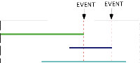
These metrics are taken from Sepkoski (1978) and Lasker (1978). The ADAPTS software uses the diversity calculation procedure of Wei and Kennett (1986). This involves weighting each taxa by the proportion of the calculation interval for which it is present. A taxon that is present for all of a calculation interval adds one to the diversity for that interval and one that is present for only half of an interval adds 0.5 to the value of diversity for that interval. Figure 1 shows a simple case. Taxon A would contribute 1.0 to the diversity of interval 4, taxon B would contribute 0.5, and taxon C would contribute 0.75. In a simple count, as used by Sepkoski (1978), diversity would be measured as 3.0. The problem with this method is that measured diversity is positively correlated wirth the arbitrarily chosen calculation interval. The Wei and Kennett (1986) method gives a diversity of 2.25. Once the diversity, D, has been recorded the number of originations (S), and extinctions (E) within each interval are calculated. On Table 1, S=3.0 for interval 4, S=1.0 for interval 3 and S=0.0 for interval 2. The values for E are 2.0, 0.0 and 2.0 for the same intervals. The ADAPTS software allows the user to set the calculation interval to whatever values are appropriate.

Rate Calculations. A rate calculation is a measure of the amount of change in a variable in a given interval of time. The values of D, S and E are used to calculate the taxonomic evolutionary rate metrics, using the following equations from Sepkoski (1978) and Lasker (1978);

• Rate of Speciation (r_s). r_s = 1/D x S/delta t (1)
• Rate of Extinction (r_e). r_e = 1/D x E/delta t (2)
• Rate of Diversification (r_d). r_d = r_s - r_e (3)
• Rate of Turnover (r_t) (Lasker (1978). r_t = r_s + r_e (4)
• Rate of Change in Diversity (delta D). delta D = r_d x D (5)

Raup and Boyajian (1988), Benton (1995), and Jablonski (1995) considered the various methods of quantifying extinction rates, but their comments apply to all diversity related metrics. They observed that using the absolute number of extinctions per interval is flawed, as it fails to take into account the number of taxa present. Correcting for diversity introduces errors in diversity estimation. Using a per interval approach (E/t) introduces timescale errors. Per taxon rates are in favour amongst theoreticians (Raup and Boyajian 1988; Gilinsky 1991; Hallam and Wignall 1997) and give a probability of extinction for each taxon in each period. However, this method combines the problems of errors in diversity and timescale measurements. Pease (1985, 1988a, 1988b, 1992) has considered potential problems with the mathematical expressions used in the calculation of extinction rates. Pease notes that as diversity, the denominator, approaches zero more rapidly in the geological past than the number of extinctions, the numerator, which could cause the reported decline in extinction rate as the Recent is approached, because dividing by a smaller denominator will give in a larger result. Pease (1992) pointed out that the "Pull of the Recent" (Raup 1979) could compound the problem, by inflating diversity close to the Recent, which could result in an artificial decline in extinction rates due to inflated estimates of diversity.

Survivorship Analysis

All methods of survivorship analysis used by ADAPTS require the generation of life tables (see Table 2). The first column shows the age classes, the second column contains the number of taxa that went extinct in that interval, the third column shows the survivors at the start of the interval, and the final column is the extinction rate for that interval. The mortality rate is calculated with the expression q_x = d_x/l_x. This example was designed to show a constant probability of extinction. The survivorship curve is constructed as a log-linear plot of age class against the log of the number of survivors at the start of each interval, after Van Valen (1973a). Van Valen proposed "The Law of Constant Extinction" based upon the linear nature of the survivorship curves that he generated from data. Linearity implies a constant rate of extinction and hence the probability of extinction of a taxon should be invariant with respect to its age.

Raup (1975) named this hypothesis "Van Valen's Law". However, he also noted that there were some methodological problems with Van Valen's analysis. Raup's analysis of the ammonoid Family data indicated a nonlinear extinction pattern, as shown by his use of Epstein's Test. In trying to account for the discrepancy Raup observed that although the first x value in life tables is 0.0, most of Van Valen's plots do not start at 0.0, but at 1.0, effectively underweighting the lack of extinctions amongst short lived taxa. Raup manipulated the ammonoid Family data by adding a number of short-lived taxa and this modified data "passed" Epstein's Test. Sepkoski (1975) demonstrated that the distribution of stage lengths was log-normal with a positive skew (Sepkoski 1975; Figures 1 A-D). Plotting survivorship curves on this framework generated curves with flat tops and near-linear sloping limbs (Sepkoski 1975; Figures 2 A-C). Many of Van Valen's plots have this shape. Modern timescales, such as Harland et al. (1990), try to standardize stage lengths, thus removing much of this bias. Sepkoski also estimated the preservation potential of the shape of survivorship curves and found that it was possible for the true shape to be reconstructed with only 20% of taxa in a group, if preservation potential was sufficiently high (>97%). However, once preservation potential started to decrease, the shape became distorted, unless sampling improved. This effect was most pronounced for concave survivorship curves, that recorded an age-decreasing risk of extinction.

Corrected Survivorship Score (CSS). One of the drawbacks of the dynamic survivorship method is that for the shape of the curve to reflect an age-dependent pattern extinction rates must be stochastically constant in real time. To correct for variation in real time extinction rates, Pearson (1992, 1995) introduced the CSS. The CSS is calculated with this formula:

CSS = L x R_e (extant)/R_e (total) (6)

where L is the longevity of the taxon, Re (extant) is the average rate of extinction for the duration of the taxon and Re (total) is the average rate of extinction for the whole dataset. The CSS for each taxon is calculated and then the survivorship analysis proceeds as normal. As R_e (extant) and R_e (total) are required to calculate the CSS, ADAPTS will automatically engage the taxonomic diversity routines if the user requests the CSS.

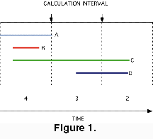
Extinction Intensity Survival Score (EISS). The use of time-averaged rates for examining patterns of extinction presents a problem. Although the time when an extinction took place is instantaneous, its influence is spread across the whole calculation interval. Taxa that originate after, or go extinct before, an event, but within the same calculation interval, are treated as though they were present during the event, thus adding "noise" to the CSS calculations. Pearson (1995, p. 122) suggested a refinement of the CSS, whereby longevity is measured in extinction events survived, with each extinction event adding 1/D to the longevity of each taxon surviving the event. This is basically equivalent to the CSS, except it has the advantage of cutting down the "noise" arising from not specifiying the order of extinctions in each calculation interval. This method scores each taxon by of the number of extinctions it survives. The general scoring procedure follows (Figure 2):

• The taxon adds 0 to its EISS. A does not increase its EISS, while, as diversity is 3 at the time of A's demise B and C both add 1/D = 1/3. When B becomes extinct B adds 0 whereas C adds 1/2. In this simple case, the EISSs for B and C are 1/3 and 5/6 respectively.
• The taxon that goes extinct scores 0. All other taxa extant at the time of the event score 1/D. In this example, both B and C survive the extinction of A. A gains an EISS of 0.0, while, as diversity is 3.0 at the time of A's demise B and C both score 1/D = 0.33. When B becomes extinct B scores 0.0 while C scores 0.5. The EISSs for B and C are 0.33 and 0.83 respectively. Although B is much shorter lived it has an higher EISS, as it outlived A.

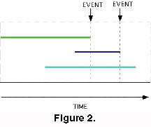
There is the special case in which two or more taxa go extinct simultaneously. This requires a modified procedure. This is illustrated in Figure 3.

• The diversity is calculated for the instant of the extinction event.
• In Case A the victims are awarded the mean score for all the taxa involved. Taxa A, B and C have the same LAD and each one scores (0+2/3+1/2)/3. The reasoning behind this is that although all three taxa have the same LOD, its is assumed that there is an order to the extinction of the three taxa, but that the order is unknown

Any taxa that survive a multiple extinction event are scored as though the extinctions were ordered, as in Case B . If a fourth taxon D is present the EISS for A, B and C would now be (0 + 2/4 +1/3)/3. D would score 1/4+1/3+1/2. This is consistent with the statement that the extinctions are ordered, but the order is unknown.

The scoring methods presented here are not the only options. Another way of handling multiple extinctions would be to give a score of 0 to every taxon that becomes extinct during a multiple event. However, this would act only to systematically lower the scores of these taxa by a uniform amount, affecting the slope, but not the linear/nonlinear nature of the survivorship curve.

Epstein's Total Life Method (Epstein's Test). Test 3 of Epstein (1960a), is better known as Epstein's Test in the palaeontological literature, after its use by Raup (1975). It is a statistical method for determining whether survivorship curves are linear. Epstein's Test has been used in several previous studies, but some of these contain misprints of the actual equations (Wei and Kennett 1983; Pearson 1992, 1995, 1996). We also note that the program previously used by Pearson (1995) contained an error that caused the volume presented for the total lives to be inflated, but did not affect the efficacy of the test or the interpretation of the results. However, this error does not affect the scientific conclusion of that earlier work. Reference to Epstein (1960a) or Raup (1975) is recommended. The "total life" of a taxon is the summation of the longevities of all taxa that become extinct before the taxon becomes extinct. Longevities are ranked as shown below:

d₁=< d₂=<....=<d_r

The total lives (T) are calculated as follows;

T₁ = rd₁
T2 = d₁ + (n-1)d₂
T₃ = d₁ + d₂ + (n - 3 +1)d₃
....
Tr = d₁ + d₂ + ...+ (n - r +1)d_r (7)

To illustrate how the calculations are done take T₃ above and let n = 50, d₁ = 5 d₂ = 6, and d₃ = 7;

T₃ = 5 + 6 + (50 - 3 +1) x 7
= 5 + 6 + (48 x 7)
= 347

If the taxa under consideration exhibit linear survivorship, Epstein (1960a) proved that the sum of (r - 1) total lives will have a normal distribution. The theoretical mean is calculated thus;

(r-1)T_r / 2 (8)

Standard deviation is calculated by;

[ (r-1)T_r²/12]^1/2 (9)

The null hypothesis is tested by comparing the sum of (r-1) lives with the theoretical range, calculated thus;

theoretical mean ± (1.96) x standard deviation (10)

If the sum of (r-1) lives lies within the theoretical range, then the null hypothesis of duration-independent extinction is accepted at the 5% significance level. A worked example from Epstein (1960b) verified that ADAPTS carries out this test correctly.

The use of Epstein's Test removes the subjectivity of "fitting a line" on the survivorship curve. Cumulative curves can look very regular and thus be interpreted as linear by those unused to viewing them (Raup, 1975). However, statistical methods are not infallible and there will be cases where slightly nonlinear curves will pass as linear. Hoffman and Kitchell (1984) found that Epstein's Test can be sensitive to variation in the lower right hand portion of a survivorship plot, and that, for both simulated and real data sets, this could result in a curve that is linear for all but the last few points to be assessed as non-linear by Epstein's Test.

Ancestor-Descendant (A-D) Tests

The following tests are the ancestor-descendant (A-D) tests of Pearson (1998). They are used to quantify asymmetry in phylogenetic trees. The premise of the tests is that if there have been systematic variations in rates of extinction and/or speciation in a group this has the potential to be recorded as tree asymmetry.

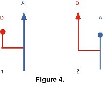A-D Extinction Test. This test is concerned with whether the ancestor or descendant of an A-D pair tends to go extinct first. The LODs of the pair are compared to see which one became extinct first. There are four possible outcomes (Figure 4):

1. Ancestor outlives descendant. (Figure 4, 1);
2. Descendant outlives ancestor. (Figure 4, 2);
3. Simultaneous extinction;
4. Indeterminate, as ancestor is unknown.

Only nodes that exhibit the first two cases are summed and subjected to a chi-squared analysis. If evolution is random then no statistically significant departure from the null hypothesis (that in half of the cases the ancestor should die before the descendant and vice versa) should occur.

Survivorship Control Test. This test represents a "control" on the A-D extinction test. If a pattern of age-dependent extinction exists in the data this would skew the chi-squared result. If this restricted test produces a similar chi-squared result then the age-dependency pattern is probably responsible for the bias (Pearson 1998). Each taxon is randomly assigned a new ancestor from the set of all taxa that were present at its time of origin. This procedure can select the actual ancestor as the random ancestor. Taxa whose ancestor is unknown retain this status, as it is assumed that there is a good taxonomic reason for this status. The altered data set is then analysed as above.

A-D Speciation Test. This test also compares A-D pairs, but in this case to look for bias in patterns of origination. All taxa in the tree are examined in turn and checked to see whether the taxon is descended from the ancestor or descendant of the previous branching event. This generates four possible outcomes (Figure 5):

1. Descended from a descendant (Figure 5, 1);
2. Descended from an ancestor (Figure 5, 2);
3. Unknown, due to ancestor being unknown;
4. Unknown, due to the ancestor of the A-D pair being subject to Case 3 above.

As in the A-D extinction test, only cases 1 and 2 are used in the chi-squared calculation. The null hypothesis is that both members of the A-D pair are equally likely to give rise to new taxa in future.

A-D Speciation Test (Restricted). The speciation and extinction tests are not necessarily independent of each other. If a strong pattern emerges in the extinction test, this would result in a systematic bias in the speciation test. Greater longevity would result in more chances to give rise to daughter taxa, due to the fact that the surviving taxa are systematically longer-lived (Pearson 1998). To investigate this possibility the A-D speciation test (restricted) is used. The "restriction" criterion is that both the ancestor and descendant of the previous branching event must survive until the appearance of the third taxon. Cases in which this criterion is not met are excluded from the chi squared test. The possible cases for a taxon are:

1. Descended from descendant, with both ancestor and descendant of the previous branching still in existence. (Figure 5, 1);
2. Descended from ancestor, with both ancestor and descendant of the previous branching still in existence. (Figure 5, 2);
3. Indeterminate, due to ancestor being unknown;
4. Indeterminate, due to the ancestor of the A-D pair being subject to case 3 above;
5. Indeterminate due to the extinction of either the ancestor or descendant of the previous branching (Figure 5, 3-4).

Random Branching Model

To verify the ability of ADAPTS to detect known random patterns, a program for generating random phylogenetic trees, TREE GROWTH, was written, which can be found in Appendix 2. The power of stochastic models to generate patterns that resemble those from the fossil record was first highlighted by Raup et al. (1973) and has become a major area of interest, although the most ambitious attempt at interpreting the history of clades as random walks (Gould et al. 1977) was refuted by Stanley et al. (1981). The TREE GROWTH software uses a model in which the probabilities of speciation and extinction are constant, based upon the time homogeneous models of Simberloff et al. (1981), Raup (1985) and Pearson (1998). Such models are know as time homogeneous models. This program started with one taxon in the "clade" and the probabilities of branching and extinction were set at p=0.01. If a new taxon arose at time t, its ancestor was noted and it was then subjected to the branching/extinction algorithm at time t+1. A target zone for the number of taxa was defined and the program was designed to return only trees in which all taxa were "extinct" by the time the target number of taxa was reached, to avoid problems with censorship of ranges (Furbish et al. 1990). Once a suitable tree was generated, it was analysed with ADAPTS.

RESULTS

The results of the analysis of the random tree generated by TREE GROWTH are presented here as an example of the capabilities of ADAPTS both to analyse and identify a known random dataset and to demonstrate the utility of having a program that can interface with spreadsheet/graphing packages. The tree had 986 taxa, spread across 575 myr of simulation time and was analysed in 1 myr intervals. Results are broken down into the three main areas of analysis: taxonomic evolutionary rates, survivorship and tree asymmetry tests.

Taxonomic Evolutionary Rate Results

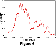Figure 6 shows the results of the diversity of the random dataset through time and serves as a reminder of the power of such random walks to produce deterministic-looking patterns!

Survivorship Results

Dynamic Survivorship. If there is no age-dependency and a stochastically constant rate of extinction, a linear survivorship curve should result. Figure 7 shows the curve for the 986 taxa and the value for Epstein's Test (Table 3) is within the expected range of values.

Corrected Survivorship. The CSS corrects for systematic variation in real time extinction rates. Fluctuations in the per taxon rate exist in the model, as Figure 7 shows. However, these are a known random signal. Since the random model contains no non-stochastic variation in the extinction rate, the CSS will not be significantly different in shape to the dynamic survivorship curve.

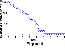
Extinction Intensity Survival Score. The EISS is shown on a different plot (Figure 8), as it is not directly comparable to the other two measures of survivorship. A linear curve from this test means that there is no variation in the probability of a taxon becoming extinct, relative to the number of extinction events that it has experienced. The EISS curve is indistinguishable for linear by Epstein's Test.

Ancestor-Descendant (A-D) Test Results (Table 4)

A-D Extinction Test. The null model expectation for this test is that there is no significant difference in the number of ancestors that become extinct before their descendants and vice versa. The result generated for this test does not depart from the null hypothesis.

Survivorship Control Test. Pearson (1998) introduced this test as a control for age-dependent effects in a dataset. If all variation in survivorship was attributable to survivorship effects then the chi-squared results for the A-D extinction test and the Survivorship Control Test should be very similar. For the random tree, this was indeed the case, suggesting that any departure from a 50:50 ratio is the result of differential survivorship. The fact that this test performed as expected on a large random dataset confirms that it is capable of discriminating between genuine bias and the effects of differential survival.

A-D Speciation Test. If there is no bias for new taxa to preferentially arise from ancestors or descendants then no departure from the null model should appear. The results from the random tree are very close to the expected 50:50 ratio.

A-D Speciation Test (Restricted). The purpose of this test is to correct for any bias introduced into the unrestricted test by the non-independence of the extinction and speciation tests. However, if there is no bias there should be no large difference between the chi-squared values for the two speciation tests. The difference is 0.01 between this test and the unrestricted test.

DISCUSSION

The preceding section has reported the results of an ADAPTS analysis of a large dataset that was randomly generated. The main purpose of this exercise was to demonstrate that ADAPTS was able to identify known random patterns. From the results, which were all well within the expected ranges, it is clear that ADAPTS is functioning correctly. By manipulating a dataset of considerable size, the speed and efficacy of ADAPTS has been demonstrated. In a study of ammonoid Families, the data set comprised 243 taxa; around a quarter of the size of this test dataset. The automation of the A-D tests has also allowed confirmation of that the two control tests are performing as predicted. This increases confidence in the results published in Pearson (1998).

While the trials of ADAPTS have been successful, the fact that the QuickBasic language is incompatible with new Macintosh operating systems is a major problem. This state of affairs necessitates a conversion of ADAPTS to another language, preferably one that is suitable for IBM-PC as well as Macintosh users. This article allows some canvassing of the palaeontological community to gauge the level of potential support that might exist for further development of such a tool. The source code for ADAPTS and TREE GROWTH is available in Appendix I and Appendix II respectively and at:

Site 1, USA
Site 2, United Kingdom.

These web locations also have a basic user manual. Any questions on the use of either of the programs should be addressed to the first author.

CONCLUSIONS

The ADAPTS software is a functional tool capable of taking much of the drudgery out of examining patterns of evolution in the fossil record. Testing of ADAPTS, through the use of a known random phylogeny has confirmed that the program functions as expected, as well as demonstrating the capability of ADAPTS to rapidly analyse large data sets.

ACKNOWLEDGMENTS

We would like to thank C.W. Stearns and R.T. Patterson for organising the session at the 1998 GSA Annual Meeting, Toronto, in which a summary of this work was presented. We are grateful to D. Henderson, M. Wills and S.J. Braddy for help with various programming matters and discussions. This manuscript was improved by comments from two anonymous reviewers. A. McGowan wishes to thank the Department of Earth Sciences, University of Bristol, where ADAPTS was written as part of a M.Sc. thesis, for extending support and facilities during the project and the Department of Geophysical Sciences, University of Chicago, where most of the paper was written. Some of this work was presented and discussed during a "Brown Bag" talk at the University of Chicago. Thanks to all those who took part in that seminar for the ensuing discussion.

REFERENCES

Benton, M.J. (ed.). 1993. The Fossil Record 2. Chapman & Hall, London.

Benton, M.J. 1995. Diversification and extinction in the history of life. Science, 268:52-58.

Epstein, B. 1960a. Tests for the validity of the assumption that the underlying distribution of life is exponential. Part I. Technometrics, 2:83-101.

Epstein, B. 1960b. Tests for the validity of the assumption that the underlying distribution of life is exponential. Part II. Technometrics,2:167-183.

Foote, M. 1997. Estimating taxonomic durations and preservation probability. Paleobiology, 23:278-300.

Furbish, D.J., Arnold, A.J. and Hansard, S.P. 1990. The species censorship problem: a general solution. Mathematical Geology, 22:95-106.

Gilinsky, N.L. 1991. The pace of taxonomic evolution, p. 158-174. In Gilinsky, N. L. and Signor, P. W. (eds.) Analytical Paleobiology. Short Courses in Paleontology, 4, The Paleonotological Society, Knoxville, Tennessee.

Gingerich, P.D. 1976. Paleontology and phylogeny : patterns of evolution at the species level in Early Tertiary mammals. American Journal of Science, 276:1-28.

Gould, S.J., Raup, D.M., Sepkoski, J.J., Jr., Schopf, T.J. M., and Simberloff, D.S. 1977. The shape of evolution: a comparison of real and random clades. Paleobiology, 3:23-40.

Hallam, A. and Wignall, P.B. 1997. Mass Extinctions and their Aftermath. Oxford University Press, Oxford.

Harland, W.B., Holland, C.H., House, M.R., Hughes, N.F., Reynolds, A.B., Rudwick, M.J.S., Satterthwaite, G.E., Tarlo, L.B.H. and Willey, E.C. 1967. The Fossil Record: A Symposium with Documentation. Geological Society of London, London.

Harland, W.B., Armstrong, R.L., Cox, A.V., Craig, L.E., Smith, A.G. and Smith, D.G. 1990. A Geological Timescale 1989. Cambridge University Press, Cambridge.

Hoffman, A. and Kitchell, J.A. 1984. Evolution in a pelagic planktic system: a paleobiologic test of models of multispecies evolution. Paleobiology, 10:9-33.

Jablonski, D. 1995. Extinctions in the fossil record, p. 25-44. In Lawton, J. H. and May, R. M. (eds.), Extinction Rates. Oxford University Press, Oxford.

Kitchell, J.A. 1990. Computer applications in palaeontology, p. 493-499. In Briggs, D. E. G. and Crowther, P. R. (eds.), Palaeobiology: a Synthesis. Blackwell, Oxford,

Lasker, H.R. 1978. The measurement of taxonomic evolution: preservational consequences. Paleobiology, 4:135-149.

Pearson, P.N. 1992. Survivorship analysis of fossil taxa when real-time extinction rates vary: the Paleogene planktonic foraminifera. Paleobiology, 18:115-131.

Pearson, P.N. 1995. Investigating age-dependency of species extinction rates using dynamic survivorship analysis. Historical Biology,10:119-136.

Pearson, P.N. 1996. Cladogenetic, extinction and survivorship patterns from a lineage phylogeny: the Palaeogene planktonic foraminifera. Micropaleonotology, 42:179-188.

Pearson, P.N. 1998. Speciation and extinction asymmetries in paleontological phylogenies: evidence for evolutionary progress? Paleobiology, 24:305-335.

Pease, C.M. 1985. Biases in the durations and diversities of fossil taxa. Paleobiology, 11:272-292.

Pease, C.M. 1988a. Biases in total extinction rates of fossil taxa. Journal of Theoretical Biology, 130:1-7.

Pease, C.M. 1988b. Biases in per-taxon origination and extinction rates of fossil taxa. Journal of Theoretical Biology, 130:9-30.

Pease, C.M. 1992. On the declining extinction and origination rates of fossil taxa. Paleobiology, 18:89-92.

Raup, D.M. 1975. Taxonomic survivorship curves and Van Valen's Law. Paleobiology, 1:82-96.

Raup, D.M. 1979. Biases in the fossil record of species and genera. Bulletin of the Carnagie Museum of Natural History, 13:85-91.

Raup, D.M. 1985. Mathematical models of cladogenesis. Paleobiology, 11:42-52.

Raup, D.M. and Boyajian, G.E. 1988. Patterns of generic extinction in the fossil record. Paleobiology, 14:109-125.

Raup, D.M., Gould, S.J., Schopf, T.J.M., and Simberloff, D.S. 1973. Stochastic models of phylogeny and the evolution of diversity. Journal of Geology, 81:525-542.

Sepkoski, J.J., Jr. 1975. Stratigraphic biases in the analysis of taxonomic survivorship. Paleobiology, 1:343-355.

Sepkoski, J.J., Jr. 1978. A kinetic model of Phanerozoic taxonomic diversity I. Analysis of marine orders. Paleobiology, 4:223-251.

Sepkoski, J.J., Jr. 1982. A compendium of fossil marine families. Milwaukee Public Museum Contributions to Biology and Geology, 51:1-125.

Sepkoski, J.J., Jr. 1992. A compendium of fossil marine families, second edition. Milwaukee Public Museum Contributions to Biology and Geology, 83:1-156.

Simberloff, D., Heck, K.L., McCoy, E.D. and Connor, E.F. 1981. There have been no statistical tests of cladistic biogeographical hypotheses, p. 40-93. In Nelson, G. and Rosen, D. E. (eds.), Vicariance Biogeography: A Critique. Columbia University Press, New York.

Smith, A.B. 1994. Systematics and the Fossil Record: Documenting Evolutionary Patterns. Blackwell, Oxford.

Stanley, S.M., Signor, P.W., Lidgard, S. and Karr, A.F. 1981. Natural clades differ from "random" clades: simulations and analyses. Paleobiology, 7:115-127.

Van Valen, L. 1973a. A new evolutionary law. Evolutionary Theory,1:1-30.

Wei, K-Y. and Kennett, J.P. 1983. Nonconstant extinction rates of Neogene planktonic foraminifera. Nature, 305:218-220.

Wei, K-Y. and Kennett, J.P. 1986. Taxonomic evolution of Neogene planktonic foraminifera and palaeoceanographic relations. Paleooceanography, 1:67-84.