FIGURE 1. Location map of localities mentioned in the text. For detailed locations of Manuherikia Group and Gore Lignite Measures, see Pole (2007, 2008).
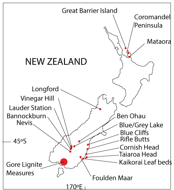
FIGURE 2. A graphic explanation of the drought estimate method derived from Walter and Lieth (1967) Klimadiagramme. The two graphs are drawn according to the protocols used by those authors. Monthly rainfall averages are indicated by the filled and blockier curves. They relate to the totals (in mm) on the right-hand side of each graph. Monthly temperature averages are indicated by the smoother line and relate to the totals (in C) on the left-hand side of each graph. Critically, a monthly temperature average (in C) is considered to be equivalent to approximately twice that figure in rainfall (in mm). Where the rainfall curve drops below the temperature curve (lightly shaded area), evaporation is estimated to be more than precipitation, and therefore there are drought conditions. In this paper the area below the curve is used as an estimate of rainfall deficit. However, the method does not distinguish between a protracted but light drought (graph at left) and a short but hard drought (middle graph). The graph at right shows rainfall precisely keeping up with evaporation for a MAT of 17°C that fluctuates within a 6°C range. To remain ‘everwet’, annual rainfall would only need to be about 400 mm.
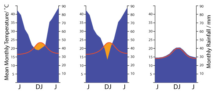
FIGURE 3. Distribution of earlyearliest Miocene plant taxa mentioned in this paper, by location. Taxa that are ubiquitous in the pollen record, such as the Nothofagus ‘types’, are not indicated and due to the difficulty of identifying some conifer pollen to genus, the records here dare based only on macrofossils. Records follow Campbell and Holden (1984), Pocknall and Mildenhall (1984), Mildenhall and Pocknall (1989), (Pole, 1993a, 1993b, 1993c, 1993d, 1993e, 1993f, 1993g, 1993h, 1993i, 1996, 2007a, 2007b, 2008, 2010a, 2010b), Pole and Douglas (1998), Bannister et al. (2005), Pole et al. (2008), Lee et al. (2007, 2010), Jordan et al. (2011, their record of Podocarpus is not accepted here as the monocyclic stomatal form and mode of papillae clearly place the fossil in Cupressaceae), and Conran et al. (2013).
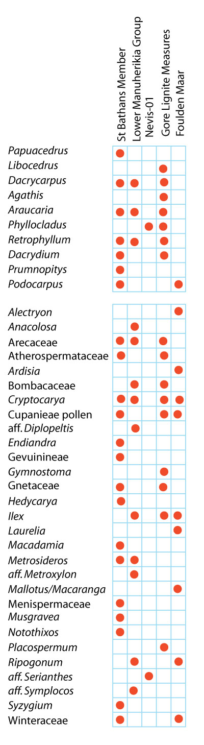
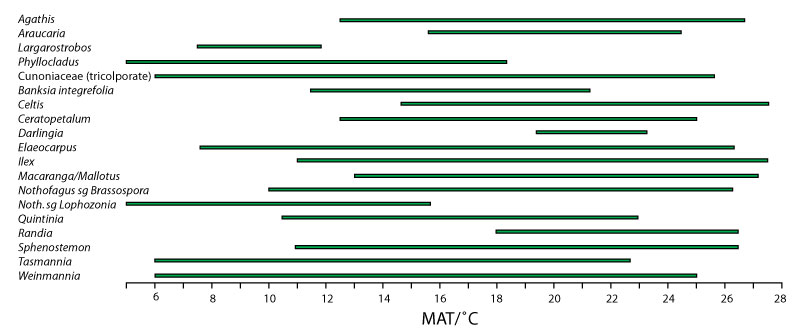
FIGURE 4. Mean Annual Temperature (MAT) ranges of selected plant taxa either known or proposed from the early to earliest middle Miocene in southern New Zealand derived from GBIF data. The bars indicate the 0.02-0.98 percentile range. Taxa not shown here include some with very broad climate ranges and those confined to New Zealand or New Caledonia as their temperature ranges are likely to be geographically attenuated. Note that within Bombacaceae the unshaded rectangle is the range for Bombax .
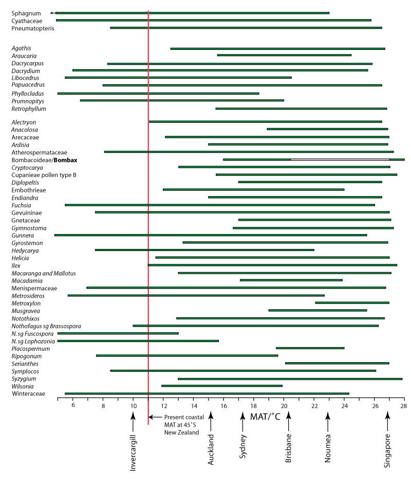
FIGURE 5. Growing Degree Month (GDM) ranges derived from GBIF data (0.02-0.98 percentile) for early-earliest middle Miocene plant taxa from New Zealand. GDM is the total of the average monthly MAT for all monthes where MAT > 10°C. For context the GDM of some key cities is shown.
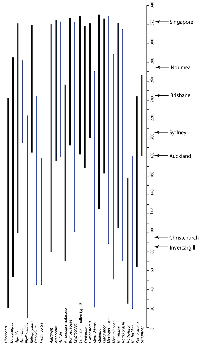
FIGURE 6. Minimum temperature of the Coldest Month ranges derived from GBIF data (0.02-0.98 percentile) for early-earliest middle Miocene plant taxa from New Zealand. For context the Minimum temperature of the Coldest Month of some key cities is shown.
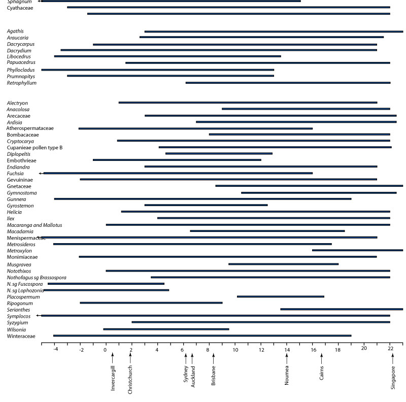
FIGURE 7. Rainfall deficit ranges derived from GBIF data (0.02-0.98 percentile) for early-earliest middle Miocene plant taxa from New Zealand and calculated using the Walther-Lieth Klimadigramm as above method. Where taxa grow in a region which has no period of rainfall deficit according to this method, it is deemed ‘everwet’. This appears as a bar of arbitrary length on the right of each range. When a range includes rainfall deficit, the degree is indicated by the ‘amount’ in mm.
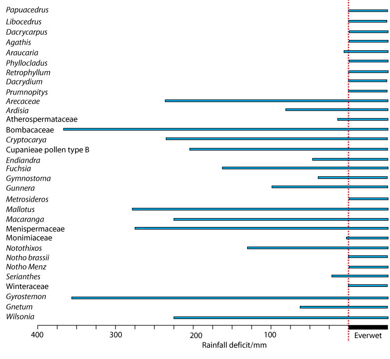
FIGURE 8. Leaf length, width, and size histograms for early-earliest Miocene leaf fossil assemblages. Size is estimated from length x width x 0.667 (Cain and Castro, 1959) and binned according to the classes in Webb (1959).
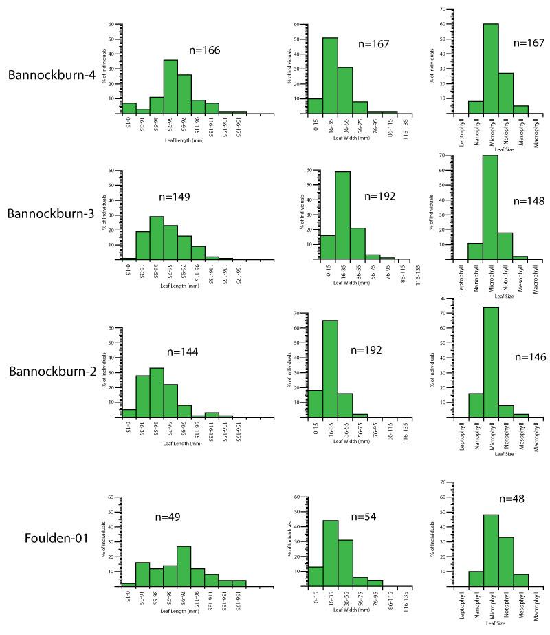
FIGURE 9. Leaf length, width, and size histograms for early-earliest Miocene leaf fossil assemblages. Size is estimated from length x width x 0.667 (Cain and Castro, 1959) and binned according to the classes in Webb (1959).
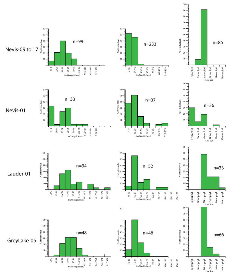
FIGURE 10. Leaf length, width, and size histograms for some extant leaf litter collections in New Zealand and Australia. Size is estimated from length x width x 0.667 (Cain and Castro, 1959) and binned according to the classes in Webb (1959).
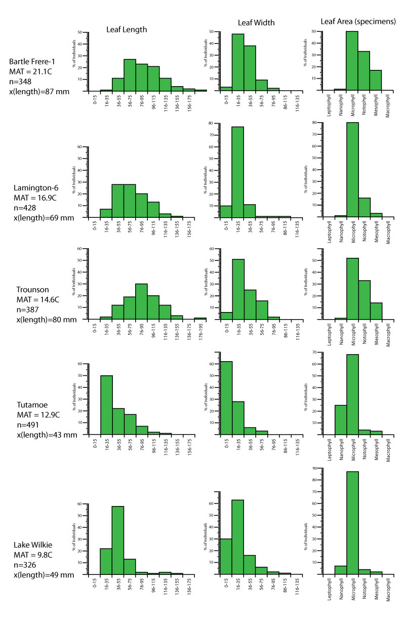
FIGURE 11. Biodiversity of fossil and recent leaf litter assemblages. Points labeled in bold to the left show the number of taxa in New Zealand early-earliest Miocene leaf assemblages versus the number of specimens. Points labeled to the left in smaller, unbold font represent extant leaf litter collections from New Zealand and Australia collected by the author. Points labeled at right in bold font are the results of extant leaf litter collections from Australia given by Greenwood (1992). The two diagonals are lines of equal biodiversity encompassing early Miocene assemblages. All points plotted on log: log axes, with MAT for extant samples in brackets.
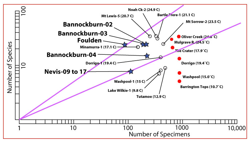
FIGURE 12. MAT ranges based on GBIF data (0.02-0.98 percentile) for taxa relevant to middle Miocene, Casuarinaceae Zone climate in New Zealand (essentially the vertebrate assemblages of the St. Bathans region).
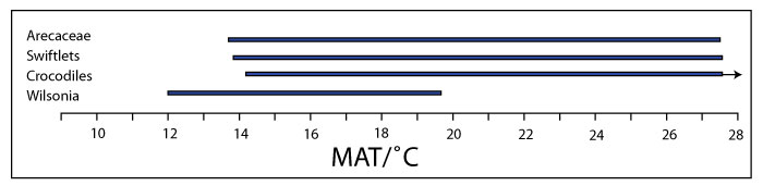
FIGURE 13. Grass charcoal from palynological preparation, middle Miocene of Mata Ck, near St. Bathans (Slide P761, Sample Mata-2, scale bar equals 20 μm).
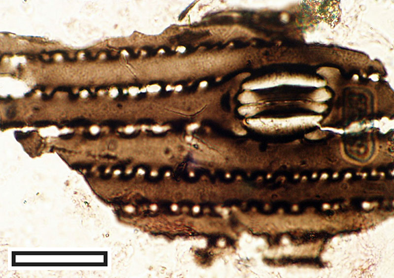
FIGURE 14. Histograms of leaf length, width, and size for the J.D. Campbell, Kaikorai Valley assemblage. Size is estimated from length x width x 0.667 (Cain and Castro, 1959) and binned according to the classes in Webb (1959).
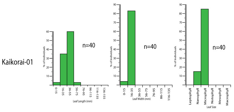
FIGURE 15. Nothofagus leaves from middle to late Miocene deposits in New Zealand. 1. Beesons Island Volcanics, Medlands Stream, Great Barrier Island (Auckland University Geology Department specimen AU4567). 2. Longford Formation, Murchison (LX1281). 3. Glentanner Formation, Ben Ohau (Canterbury Museum specimen zp298). 4. Bannockburn Formation, Vinegar Hill (LX980). Scale bar equals 10 mm.
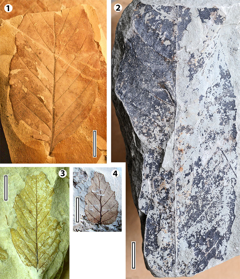
FIGURE 16. Comparison of results for MAT using different methods. Two different schemes for classifying MAT are given at left. Error bars are ± 5C for the LMA and CLAMP results and ± 2C for leaf-length.
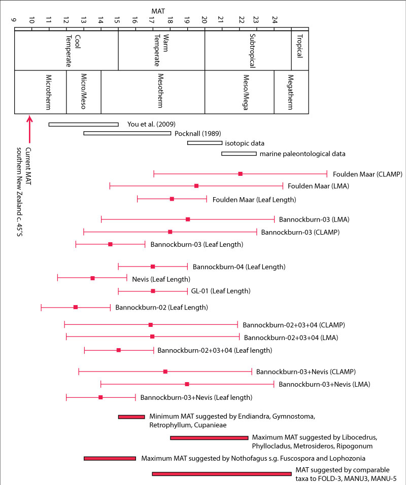
FIGURE 17. As per the International Commission on Stratigraphy (www.stratigraphy.org), the division of the Miocene into ‘early,’ ‘middle,’ and ‘late’ is no longer recognized. They are used throughout the present paper as they will remain a frame of reference for some time to come. The six international stages that now subdivide the Miocene are shown here as well as their correlation with the New Zealand local stages and series. The absolute ages for stage boundaries, and their correlation with the previous ‘Early’, ‘Middle,’ and ‘Late,’ follows Morgans et al. (2004). To the right are the Pocknall and Mildenhall (1984) and Mildenhall and Pocknall (1989) palynological zones, some comments relevant to their dating, and furthest right are the zones in Pole and Douglas (1998). All are shown with their correlation suggested here.
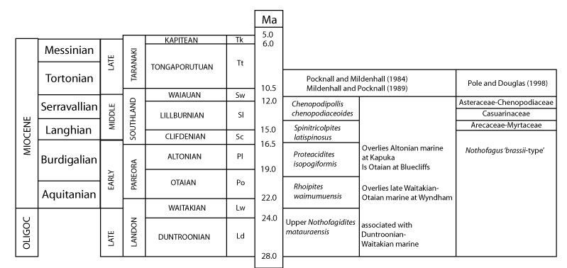
FIGURE 18. New parataxa -1. Scale bar equals 10mm. 1. MANU-36, OU13926, Bannockburn-02. 2. MANU-37, OU12955, Bannockburn-03. 3. MANU-38, OU29867, Bannockburn-03. 4. MANU-39, LX071, Bannockburn-03. 5. MANU-40, OU13792, Bannockburn-02.
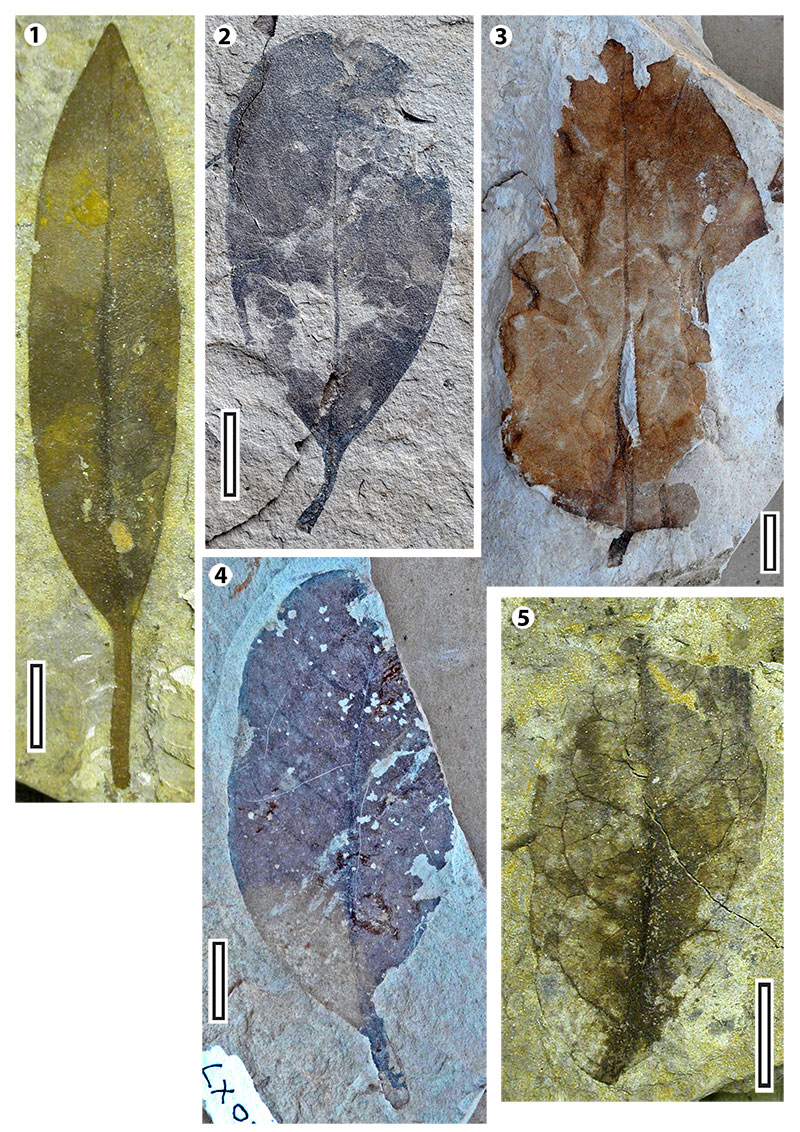
FIGURE 19. New parataxa -2. Scale bar = 10mm. 1. MANU-41, LX541, Nevis-14. 2. MANU-42, LX431, Nevis-04. 3. MANU-43, LX393, Nevis-17. 4. MANU-44, LX745, Bannockburn-03. 5. MANU-45, LX029, Bannockburn-03. 6. MANU-46, LX761, Bannockburn-03. 7. MANU-47, OU13829, Bannockburn-02. 8. MANU-48, LX115, Bannockburn-03.
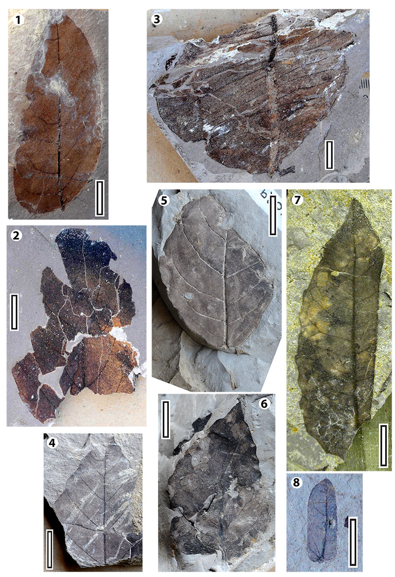
FIGURE 20. Histograms of MAT overlap for Foulden Maar taxa as listed in Reichgelt et al. (2013). The amount of overlap is indicated by the y-axis, and MAT range (rounded to nearest full degree) by the x-axis. 1. Based on range figure in Reichgelt et al. (2013). 2. Based on global range of taxa, 0.02-0.98 percentile. 3. Based on global range of data, 0.1-0.9 percentile. 4. Based on southwest Pacific data only, 0.02-0.98 percentile. 5. Based on southwest Pacific data only, 0.1-0.9 percentile.
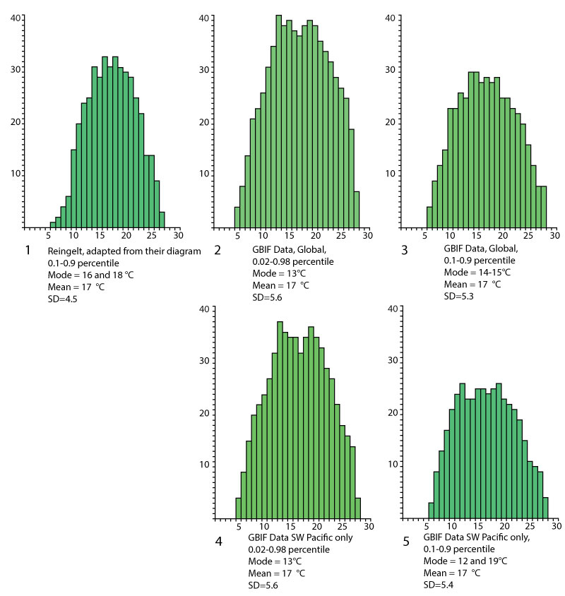
FIGURE 21. MAT ranges (0.02-0.98 percentile) of extant Podocarpus species according to GBIF data arranged according to midpoints of estimated area (in brackets after species name. See text for method).
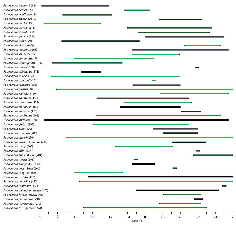
FIGURE 22. MAT ranges (0.02-0.98 percentile) of extant Podocarpus species according to GBIF data arranged according to midpoints of estimated area (in brackets after species name. See text for method.).
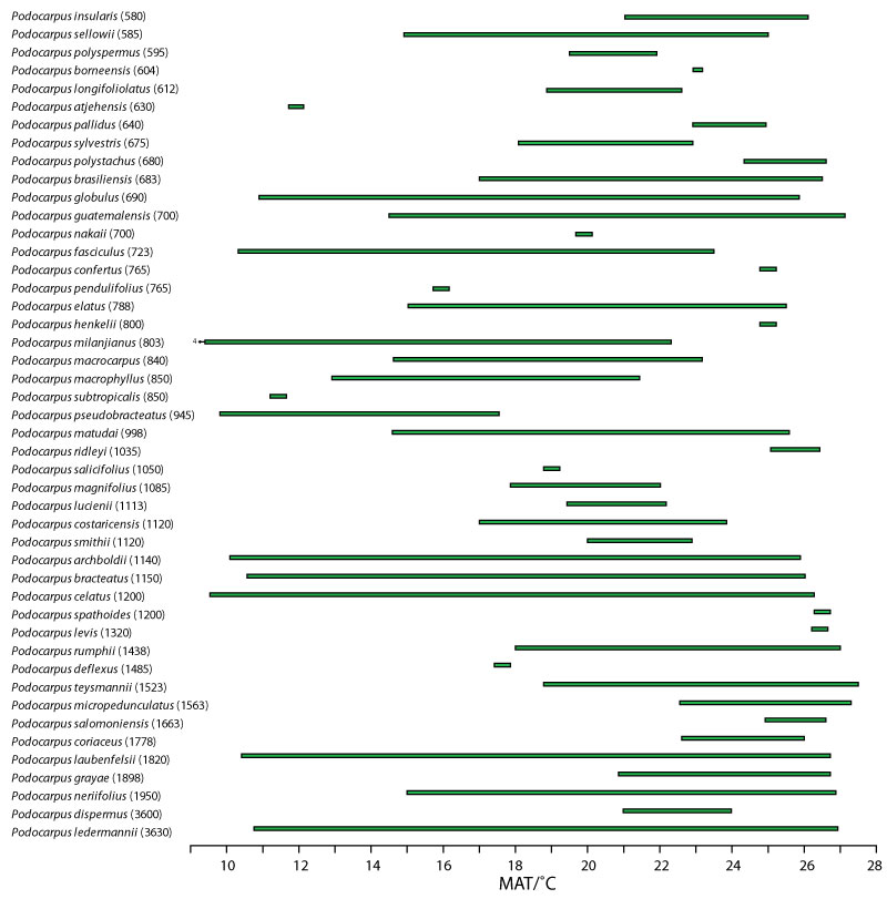
FIGURE 23. MAT ranges (0.02-0.98 percentile) of the taxa in Sluiter et al. (1995) based on GBIF records.