APPENDIX 1.
Instructions on inputting data into R using example coordinates from the outline of a brachiopod dorsal valve.
The following set of data shows input of coordinates into R using the scan command. Copy between ##START and ##END, paste into your R command, and hit enter. The objects “x” and “y” are the coordinates of successive points along a biological outline. In the case of accretionary growth, coordinates are assumed to begin at the umbo and be oriented in a counter-clockwise direction. It is important that each valve or outline has its own separate coordinates. R interprets instructions line by line with any text after a hash symbol being ignored by R and serving as a comment.
Example data from a brachiopod dorsal valve. This data input method uses the scan command, which is ideal when x and y coordinates are saved in Excel or a similar program.
1. ##START
x <-scan()
##END
2. After setting up the scan command, values are assigned to the object. Copy the following x values and paste into R. If you have your own data saved in an Excel spreadsheet, copy the x value column and paste into R.
##START
43.586104 43.661530 43.742566 43.794569 43.827071 43.827687 43.849945
43.831238 43.811462 43.765150 43.702984 43.664955 43.582932 43.514087
43.466883 43.399287 43.339617 43.266055 43.198281 43.089008 42.922561
42.805183 42.717016 42.535607 42.390088 42.238425 42.128974 41.962706
41.868394 41.724480 41.587601 41.444400 41.293806 41.149892 41.006334
40.841492 40.683686 40.497916 40.289615 40.082026 39.924220 39.723488
39.502543 39.209818 38.995373 38.716719 38.416959 38.202870 37.988068
37.845223 37.560426 37.311517 37.040433 36.784133 36.614039 36.315527
36.060118 35.868740 35.685110 35.465412 35.202434 35.003842 34.769895
34.536662 34.338070 34.075805 33.771327 33.439422 33.298717 33.108765
32.946598 32.678010 32.445133 32.120798 31.916776 31.642936 31.361525
31.065510 30.704750 30.485944 30.190285 29.900948 29.611611 29.330201
29.104895 28.795522 28.442511 28.167601 27.935437 27.639422 27.378939
27.047925 26.794121 26.597312 26.400147 26.154804 25.845075 25.579340
25.214576 24.961664 24.646682 24.394304 24.155818 23.846980 23.608317
23.293156 23.061884 22.817433 22.559269 22.321496 22.041156 21.817097
21.572290 21.313055 21.075461 20.900649 20.530277 20.299718 20.020447
19.740998 19.616325 19.337233 19.099639 18.911291 18.701838 18.471814
18.242325 17.872844 17.686102 17.519395 17.339331 17.165233 17.012062
16.824250 16.637685 16.458156 16.284593 16.125100 15.965072 15.756332
15.540378 15.464239 15.249533 14.999652 14.735521 14.583242 14.409322
14.221509 14.048837 13.931377 13.829236 13.669921 13.530821 13.413005
13.232406 13.079413 12.877530 12.766927 12.649111 12.460585 12.321663
12.161457 11.966788 11.771762 11.583771 11.340390 11.089795 10.909375
10.798415 10.597067 10.444431 10.334185 10.160621 10.072551 9.971123
9.833270 9.743417 9.577780 9.446428 9.273934 9.149974 9.026014
8.901697 8.707384 8.527320 8.333721 8.126407 7.932094 7.751852
7.558253 7.399473 7.149056 6.969527 6.837819 6.713324 6.582328
6.471547 6.375371 6.209200 6.114807 5.990668 5.845781 5.714429
5.576576 5.452616 5.329012 5.170946 5.040307 4.873957 4.728713
4.631645 4.527721 4.431011 4.335548 4.253799 4.179264
-It is important to press enter twice after pasting values in order to complete the scan command.
4. Copy the following y values and paste into R. Be sure to hit enter twice after pasting the values in order to complete the scan command. Confirm that the number of values assigned to “x” and “y” are identical. If these numbers are different, a mistake was likely made when copying and pasting values into R.
17.42193 17.50128 17.63709 17.80736 17.91378 18.16723 18.40010 18.58266
18.80744 18.96818 19.19891 19.31059 19.49154 19.70803 19.90395 20.07119
20.20343 20.32828 20.50256 20.64763 20.82644 21.01354 21.15914 21.37278
21.55916 21.71020 21.86230 22.03408 22.14432 22.26739 22.39064 22.48557
22.59439 22.71746 22.82645 22.94195 23.05763 23.16556 23.32923 23.46477
23.58045 23.72319 23.83023 23.99177 24.12009 24.28198 24.44334 24.55759
24.69998 24.78084 24.90737 25.00666 25.14763 25.26081 25.30578 25.41789
25.49589 25.54736 25.57087 25.62866 25.72759 25.78591 25.85038 25.88671
25.94503 26.01582 26.08555 26.12641 26.12285 26.11803 26.12800 26.17047
26.19273 26.21267 26.20750 26.17944 26.17231 26.18593 26.25422 26.27683
26.27638 26.30425 26.33211 26.32498 26.32631 26.31143 26.35176 26.36592
26.36003 26.37365 26.37409 26.37978 26.39447 26.38244 26.38448 26.34306
26.34226 26.27216 26.22068 26.20019 26.12885 26.08725 26.05305 26.01706
25.98990 25.92559 25.88453 25.80794 25.71692 25.65458 25.60523 25.55731
25.49479 25.44598 25.37660 25.32993 25.22199 25.15279 25.06124 24.97672
24.89612 24.79753 24.72815 24.66002 24.59135 24.50105 24.38963 24.24651
24.11507 24.02636 23.90916 23.83435 23.76711 23.67788 23.53939 23.40109
23.30517 23.20961 23.13516 23.03835 22.94840 22.89719 22.75800 22.61791
22.48450 22.38208 22.30024 22.21100 22.07991 21.99245 21.85611 21.75351
21.68663 21.61325 21.51715 21.44288 21.35328 21.27304 21.19966 21.13856
21.06465 20.99723 20.90078 20.81840 20.73620 20.61739 20.50544 20.40231
20.33614 20.22545 20.13710 20.04279 19.94687 19.81088 19.64640 19.53027
19.46463 19.33372 19.23888 19.10075 18.99201 18.88327 18.78860 18.67808
18.56088 18.42222 18.26913 18.15861 18.04845 17.90978 17.78608 17.66710
17.52879 17.44802 17.36039 17.25147 17.17826 17.08431 16.97450 16.81020
16.70849 16.59219 16.49734 16.38121 16.27247 16.14966 15.99782 15.87483
15.77206 15.66982 15.61105 15.54505 15.47220 15.35011 15.24244 15.12791
This creates a basic graph using the objects x and y. Confirm that the umbo is located at the right and the outline curves in a counter-clockwise direction. (Note: in this example the outline is oriented in the correct direction). If this is not the case, you must reverse either the x coordinates or y coordinates, or both. To reverse the x coordinates, enter the code:
To reverse the y coordinates, enter the code:
APPENDIX 2.
Instructions on generating a biological outline in R.
The following directions assume you have already defined the objects “x” and “y” using the brachiopod dorsal valve coordinates from appendix 1. Directions are included on how to modify the following code to suit your own data. Copy and paste the following code between ##START and ##END into R, then hit enter. Descriptions of the commands follow the code itself.
-This loads the package “MASS”, which is required for future commands.
-This plots a basic outline of the valve using equal units on each coordinate axis. No scale bar is shown with this plot; it is just a quick confirmation on whether the outline appears correct.
-This creates a default scale bar. “side=1” means that the scale bar is oriented parallel to the x-axis. This can be changed to “side =2”, which orients the scale bar parallel to the y-axis. “line= -8” is the spatial placement of the scale bar relative to the x-axis. Decreasing this number moves the scale bar up and increasing this number moves it down.
-Now that you know where the scale bar should be placed, you can edit the length and labels. Exit the graphics window, and enter the following four lines of code into the command window. The following code assumes you are using the brachiopod dorsal valve data from Appendix 1.
eqscplot( x, y, axes = FALSE )
axis( 1, at = c(25,35), labels = c("0 mm", "10 mm"), tck = 0.02, line = -8)
axis( side = 1, at=30, labels = F, tck = 0.016, line=-8)
axis( 1, at =seq(25,35,1), labels=F, tck = 0.009, line=-8)
-The first line of code plots the biological outline of the brachiopod dorsal valve.
-The second line of code adds length, horizontal placement, and labels to the scale bar. “at=c(25,35)” means that the scale bar will extend from x=25 to x=35. In this case, the scale bar will be 10 units long and should be labeled accordingly. “labels=c(“0 mm”,”10 mm”)” labels the tick marks at the ends of the scale bar. At x=25, the scale bar label is “0 mm”, and at x=35, the scale bar label is “10 mm”. You can change these numbers to suit your own scale bar units. “tck=.02” creates a tick mark that extends in the upwards direction because it is positive. To make it extend downwards instead of upwards, make the value negative instead of positive. To increase the length of this tick mark, increase the magnitude of the value listed after “tck= ”.
-The third line of code creates a tick mark halfway through the scale bar because in this example, x=30 is the point midway between 25 and 35. “tck=.016” creates a tick mark that extends in the upwards direction and is shorter than the end tick marks. If you do not want a halfway tick mark on your scale bar, delete this line of code.
-It is important that the number you used for the line placement of the scale bar (“line = -8”) is the same as the line placement of the tick marks so they overlap each other.
-The last line of code creates minor tick marks at every unit. “at=seq(25,35,1)” means that the ticks will be placed over the span of x=25 to x=35, with 1 unit of space in between ticks. “tck=0.009” means that the tick marks will extend upwards and they will be shorter than the end and halfway tick marks.
-It is important to save the scale bar code you just determined in a document so that it is easily accessible in step 2.
Step 2: Making a biological outline with a scale
Copy and paste the following code between ##START and ##END into R, then hit enter.
specimen.df <- data.frame( x,y)
-This combines the two objects “x” and “y” into a single data frame.
-This creates a copy of the data and saves it under the name “z.df” in case a mistake is made.
-This creates a new graphic window.
eqscplot( z.df$x, z.df$y, type="p", pch=16, cex=0.3, col=2, xlab="", ylab="", axes=F)
-This creates a plot using the data frame z.df. “z.df$x” means that the x values from the data frame “z.df” are being used in the plot. “z.df$y” means that the y values from the data frame “z.df” are being used in the plot. “pch=16” creates data points that are solid dots. Altering the value after “pch =” changes the style of data points (e.g., squares, diamonds, open circles). “cex=0.3” indicates the size of these data points. Increasing this value increases the size of the data points and vice versa. “col=2” indicates the color of the data points (e.g., 1 = black, 2 = red, 3 = green, 4 = blue). “xlab=””” and “ylab=””” means that labels on the x and y axes are absent. “axes=F” makes the x and y axes lines disappear completely.
-Now, you should have a biological outline with no labels or axes.
5. The next step is to add a scale bar to the biological outline. If you are working with the brachiopod example coordinates from appendix 1, select, copy and paste the following commands into R. The following code was determined in step 1.
axis( 1, at = c(25,35), labels = c("0 mm", "10 mm"), tck = 0.02, line = -8)
axis( side = 1, at=30, labels = F, tck = 0.016, line=-8)
axis( 1, at =seq(25,35,1), labels=F, tck = 0.009, line=-8)
-Now, you should have a biological outline with a correct scale bar.
APPENDIX 3.
R code necessary to create spiral deviation graphs.
Acquiring spiral deviations requires the function, fit.any.spirals, that in turn uses up to seven other functions. All eight functions are provided below. Select, copy and paste the functions listed in between ##START and ##END into your R session. Appendix 4 shows how to use these functions on example coordinate data. When exiting R, save the session so the functions are retained in your designated workspace.
start.angle <- function(xc, yc, u1, v1)
start.theta <- atan(abs((yc - v1))/abs(xc - u1))
# now check the starting quadrant of outline
if(xc - u1 < 0 && yc - v1 > 0) start.theta <- pi - start.theta else
if(xc - u1 < 0 && yc - v1 < 0)
start.theta <- pi + start.theta
else if(xc - u1 > 0 && yc - v1 < 0)
start.theta <- 2 * pi - start.theta
# otherwise retain the first quadrant as the start of outline
## end of function to calculate the angle from given location to the first outline coordinate
cumulative.angle.fcn <- function (x, y, u, v)
# accumulates sequential angle between coordinates (x,y) about an axis location (u,y)
xy.r <- sqrt((x - u)^2 + (y - v)^2)
x.unit <- (x - u)/xy.r # unit vector in x direction
y.unit <- (y - v)/xy.r # unit vector in y direction
npts <- length(x.unit) # number of coordinate points
theta <- acos(abs(x.unit[1:(npts - 1)] * x.unit[2:npts] +
y.unit[1:(npts - 1)] * y.unit[2:npts]))
# check whether part of the outline regresses creating negative angles
# if negative then change the sign of the angle increment
check1 <- rotate.fcn(x = x.unit[1:(npts - 1)],
y = y.unit[1:(npts - 1)], theta = -theta[2:npts])
theta.sign <- ifelse(check1.x < eps & check1.y < eps, 1, -1)
} ## end of function to accumulate angle about location
rotate.fcn <- function (x, y, theta, u = 0, v = 0)
# rotates coordinates by an angle theta about an axis location (u,v)
xp <- xx * cos(theta) + yy * sin(theta)
yp <- -xx * sin(theta) + yy * cos(theta)
} ## end of function to rotate points
fit.one.spiral.fcn <- function (x, y, start.u = NULL, start.v = NULL,
# fits a single spiral to sequential outline coordinates (x,y)
# using non linear regression with a supplied tolerance and set
# to a maximum of 400 iterations.
lspiral.lhs <- function(x, y, u, v) sqrt((x - u)^2 + (y - v)^2)
lspiral.rhs <- function(x, y, u, v, a, k) {
xtheta <- cumulative.angle.fcn(x, y, u, v)
spiral.fit <- nls(~lspiral.lhs(x, y, u, v) - lspiral.rhs(x, y, u, v, a, k),
trace = F, control = list(tol = tolerance.step,
maxiter = 400), start = list(u = u, v = v, a = 2, k = 0.2))
spiral.fit.coef <- coef(spiral.fit)
u1 <- as.numeric(spiral.fit.coef[1])
v1 <- as.numeric(spiral.fit.coef[2])
a1 <- as.numeric(spiral.fit.coef[3])
k1 <- as.numeric(spiral.fit.coef[4])
fit.summary <- summary(spiral.fit)
rp1 <- sqrt((x - u1)^2 + (y - v1)^2)
thetap1 <- cumulative.angle.fcn(x, y, u1, v1)
rpp1 <- a1 * exp(k1 * thetap1)
deviations <- rp1 - rpp1 # spiral deviations
start.theta <- start.angle(xc = x[1], yc = y[1], u1, v1)
rfit.a <- a1 * exp(k1 * thetap1)
arc.length <- sqrt(diff(x - u1)^2 + diff(y - v1)^2)
arc.length <- cumsum(c(0, arc.length))
xp1.a <- xp.a * cos(-start.theta) + yp.a * sin(-start.theta)
yp1.a <- yp.a * cos(-start.theta) - xp.a * sin(-start.theta)
parameters1 <- round(c(u1, v1, a1, k1,sigma1), 4)
names(parameters1) <- c("x.axis", "y.axis", "a1", "k1","error")
spiral.output <- list(parameters1, thetap1, arc.length,
deviations, r.fitted, xp1.a, yp1.a)
names(spiral.output) <- c("parameters1",
"angle", "arc.length", "deviations", "fitted", "xpred.orig", "ypred.orig")
} ## end of function to fit one spiral
fit.two.spiral.fcn <- function (x, y, m = NULL,
start.u = NULL, start.v = NULL, tolerance.step = 0.01)
# fits two spirals to sequential outline coordinates (x,y)
# the m th coordinate is the user specified change in spiral
# Nonlinear regression is used with a supplied tolerance and set
# at a maximum of 400 iterations.
lspiral.lhs <- function(x, y, u, v) sqrt((x - u)^2 + (y - v)^2)
lspiral.rhs <- function(x, y, u, v, a, k1, k2, m = m1) {
xtheta <- cumulative.angle.fcn(x, y, u, v)
a * exp(k1 * pmin(xtheta, xchange)) * exp(k2 *
u <- start.u # initial estimate of horizontal location of spiral axis
v <- start.v # initial estimate of vertical location of spiral axis
spiral.fit <- nls(~lspiral.lhs(x, y, u, v) - lspiral.rhs(x,
y, u, v, a, k1, k2), trace = F, control = list(tol = tolerance.step,
maxiter = 400), start = list(u = u, v = v, a = 2, k1 = 0.2, k2 = 0.2))
spiral.fit.coef <- coef(spiral.fit)
u1 <- as.numeric(spiral.fit.coef[1])
v1 <- as.numeric(spiral.fit.coef[2])
a1 <- as.numeric(spiral.fit.coef[3])
k1 <- as.numeric(spiral.fit.coef[4])
k2 <- as.numeric(spiral.fit.coef[5])
fit.summary <- summary(spiral.fit)
rp1 <- sqrt((x - u1)^2 + (y - v1)^2)
thetap1 <- cumulative.angle.fcn(x, y, u1, v1)
a2 <- a1 * exp((k1 - k2) * zz)
a1 * exp(k1 * thetap1), a2*exp(k2 * thetap1))
start.theta <- start.angle(xc = x[1], yc = y[1], u1, v1)
rfit.a <- ifelse(thetap1 < zz, a1 * exp(k1 * thetap1), a2 *
arc.length <- sqrt(diff(x - u1)^2 + diff(y - v1)^2)
arc.length <- cumsum(c(0, arc.length))
xp1.a <- xp.a * cos(-start.theta) + yp.a * sin(-start.theta)
yp1.a <- yp.a * cos(-start.theta) - xp.a * sin(-start.theta)
parameters1 <- round(c(u1, v1, a1, a2, k1, k2,sigma1), 4)
names(parameters1) <- c("x.axis", "y.axis", "a1", "a2", "k1","k2","error")
spiral.output <- list(parameters1, thetap1, arc.length, deviations, r.fitted,
names(spiral.output) <- c("parameters1", "angle", "arc.length", "deviations",
"fitted", "xpred.orig", "ypred.orig")
} ## end of function to fit two spirals with a given change location
plot.spiral.fit <- function( spiral.output=zzz, change=NULL, xdata=x,ydata=y, title.label ="" )
if( is.null(change) ) spirals <- 1 else spirals <- 2
x.fit <- spiral.output$xpred.orig
y.fit <- spiral.output$ypred.orig
xaxis <- spiral.output$parameters1[1]
yaxis <- spiral.output$parameters1[2]
eqscplot( xdata, ydata, pch=1, axes=F, xlab="",ylab="")
lines( x.fit, y.fit, col=2, lwd=2)
points( xaxis, yaxis, pch=10, cex=2.5,col=2)
points(xdata[change], ydata[change], pch=16, col=4, cex=1.8)
title( paste( " One Spiral"," for specimen ", title.label), cex.main=1.1, col.main=4,adj=0.0)
title( paste( " Two Spirals change at ",change[1]," for ", title.label), cex.main=1.0, col.main=4,adj=0.0)
# end of function to plot original outline and fitted spiral(s)
plot.spiral.deviations <- function( spiral.output=zzz, change=NULL, title.label ="" )
deviations <- spiral.output$deviations
arc.length <- spiral.output$arc.length
plot( arc.length, deviations, type="s", xlab="Secant or Arc length from umbo",
abline( v=arc.length[change], col=2,lwd=2,lty=3)
mtext( paste( "Spiral deviations : ", title.label), side=3, outer=T, line=-2,cex=1.2,col=4,adj=0.05)
# end of function to plot spiral deviations
## function to use the above functions and acquire spiral deviations
fit.any.spirals <- function (x, y, m = NULL, axis.start = c(NULL,NULL),
specimen = "", res1 = NULL, res2 = NULL, tolerance.step = 0.01,
plot.fit = FALSE, plot.deviations = FALSE )
# fits either one or two spirals depending on the user supplied m th coordinate
# of the second spiral. If the initial axis location is not supplied
# then the outline will be plotted and location requested through a
title("Please mouse (left) click your best guess at axis location",
cex = 0.9, col.main = 2, adj = 0)
points(xx[1], yy[1], pch = 16, col = 2, cex = 1.1)
if (is.null(m)) spiral <- 1 else spiral <- 2
if (spiral==1) { spiral.output <- fit.one.spiral.fcn(x = xx, y = yy, start.u = start.u,
start.v = start.v, tolerance.step = tolerance.step) }
else { spiral.output <- fit.two.spiral.fcn(x = xx, y = yy, m = m,
start.u = start.u, start.v = start.v, tolerance.step = tolerance.step) }
plot.spiral.fit(spiral.output = spiral.output, change = m,
title.label = specimen, xdata = x, ydata = y)
plot.spiral.deviations(spiral.output = spiral.output,
change = m, title.label = specimen)
APPENDIX 4.
Instructions on how to use the R code in Appendix 3 to generate spiral deviation graphs, using either one or two spirals.
The following are directions to plotting spiral deviation graphs, with either one or two spirals. These directions assume you have worked through appendices 1-3, and are using the brachiopod shell coordinates from appendix 1. Select, copy and paste the functions listed in between ##START and ##END into your R session.
Spiral deviations using one spiral
1. ##START
example.fit<- fit.any.spirals(x,y, plot.fit=TRUE, specimen="A1, one spiral" )
##END
-After entering this line of code, a cross-shaped cursor will appear and you will be asked to click the location of the spiral axis. In order to do this, magine that you place a round coin inside the curve of the umbo so that it fits perfectly. The center of that imaginary coin is the approximate location of the spiral axis where you should click. Based on your chosen spiral axis, R will choose the best location for the spiral axis. The output for this code is a spiral-fitting graph, which displays the best fit of one perfect spiral (red line) to the biological outline.
2. ##START
example.fit <- fit.any.spirals(x,y, plot.deviations=TRUE, specimen="A1 example")
##END
-Click the approximate location of the spiral axis again. The output of this code is a spiral deviation graph, which plots spiral deviation versus growth from umbo. The blue line represents a spiral deviation of zero.
3. ##START
example.fit[[1]]
##END
This code displays the spiral output, which includes x.axis, y.axis, a1, k1, and error. “x.axis” and “y.axis” are the coordinates of the spiral axis location. “a1” is the distance between the spiral axis and the first coordinate pair at the umbo. “k1” is the spiral parameter, which indicates the shape of the valve. Higher values are associated with flatter valves and lower values are associates with more rounded valves. “error” is an indicator of how well the perfect spiral fits the biological outline. Lower values (<0.2) are preferable to higher values, and indicate a better spiral fit.
Spiral deviations using two spirals
1. #START
example.dorsal1<- fit.any.spirals(x,y, m=108, plot.fit=TRUE, specimen="A1, two spirals" )
##END
-Click the approximate location of the spiral axis. This code fits two spirals to the brachiopod outline with a second spiral start location at the 108th point from umbo. “m=108” means that the second spiral starts at the 108th point from the umbo. See text for discussion of where to start a second spiral. The output of this code is a spiral-fitting graph, in which the red lines are the two perfect spirals and the blue dot is the second spiral start location.
2. ##START
example.dorsal1 <- fit.any.spirals(x,y, m=108, plot.deviations=TRUE)
##END
-Click the location of the spiral axis. This code creates a spiral deviation graph, which plots spiral deviation versus growth from umbo. The vertical red-dotted line represents the location where the second spiral starts.
3. ##START
example.dorsal1[[1]]
##END
-This code displays the spiral output, which includes x.axis, y.axis, a1, a2, k1, k2, and error. When using two spirals, “a” and “k” values are computed for each spiral.
APPENDIX 5.
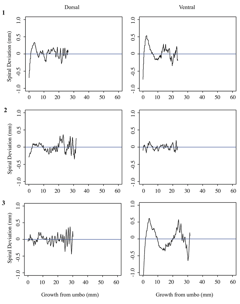
Spiral deviation graphs generated from the other halves of brachiopod shells shown in Figures 4-7.
5.1. Spiral deviation graphs generated from the corresponding halves to shells used in Figure 4 (Laqueus rubellus).
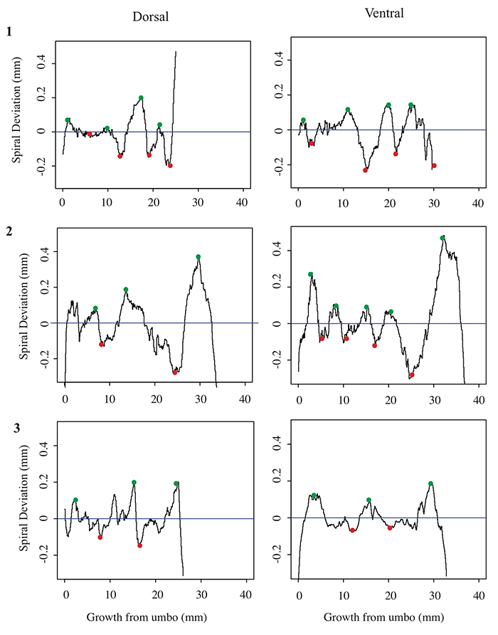
5.2 Spiral deviation graphs generated from the corresponding halves to shells used in Figure 5 (Terebratula terebratula).
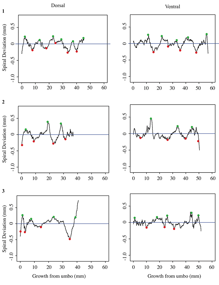
5.3 Spiral deviation graphs generated from the corresponding halves to shells used in Figure 6 (Platystrophia ponderosa).
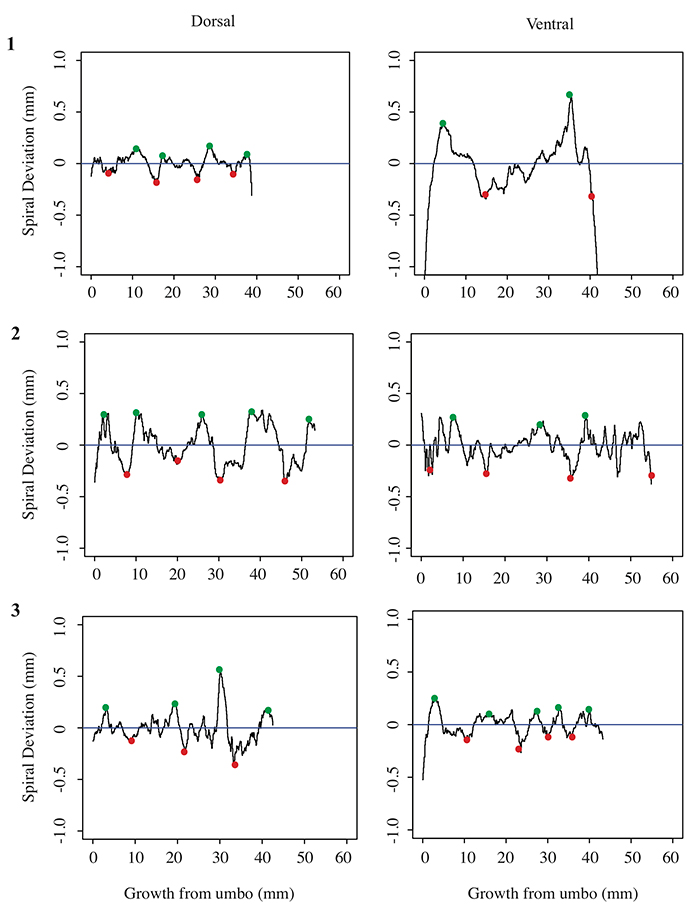
5.4 Spiral deviation graphs generated from the corresponding halves to shells used in Figure 7 (Pseudoatrypa sp.).