FIGURE 1. Geographical and stratigraphic location of the Marambio Group, James Ross Basin, Antarctic Peninsula. The stars mark the locations of the samples. (Modified from Crame et al., 2004 and Olivero, 2012).
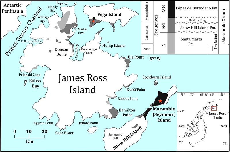
FIGURE 2. Composite range chart of Maorites species from the López de Bertodano Formation, southern Marambio Island, Antarctic Peninsula. Species are ordered by first appearance with 50% confidence interval ranges illustrated as grey lines. Although the M. densicostatus confidence interval spans the Cretaceous-Paleogene boundary, this species did not survive into the Danian. 1. M. tuberculatus; 2. M, seymourianus; 3. M. weddelliensis; 4. M. densicostatus. Abbreviations: SHI, Snow Hill Island Formation; S, Sobral Formation. (Modified from Witts et al., 2015).
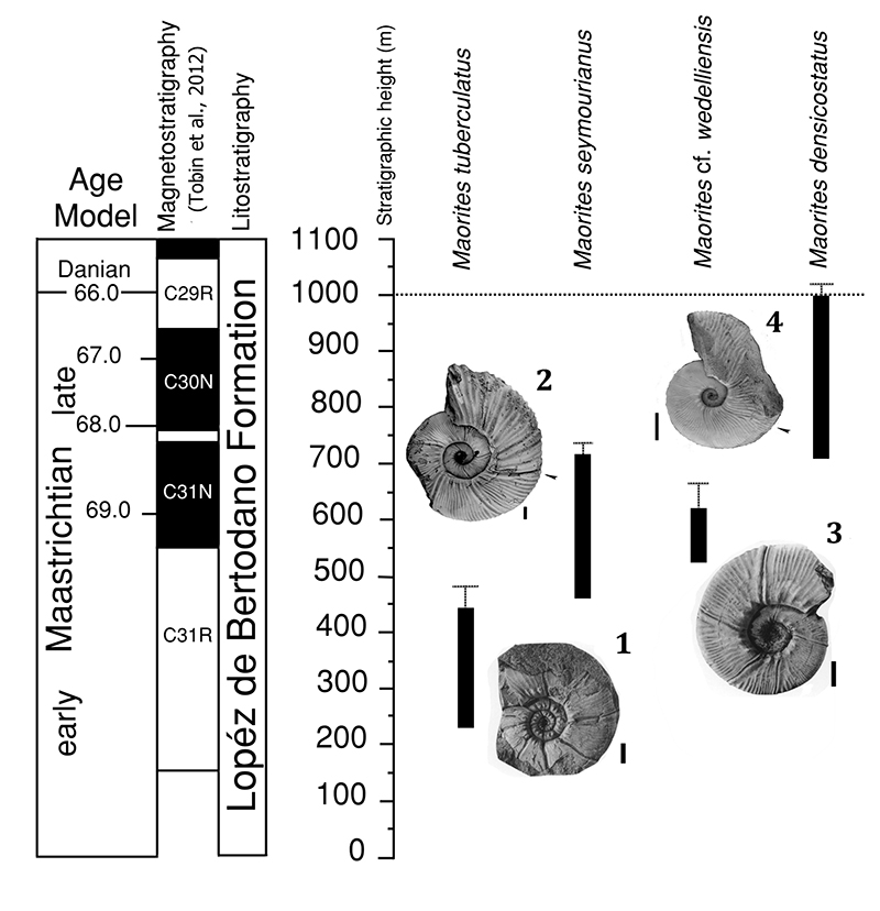
FIGURE 3. Some specimens used for this work. 1. Maorites densicostatus (CPBA-171992). 1.1: Lateral view. 1.2: Ventral view. 1.3: Apertural view. 2. Maorites seymourianus (CPBA-16814). 2.1: Lateral view. 2.2: Ventral view. 2.3: Apertural view. 3-4. Comparison between species in lateral view. 3. M. densicostatus (CPBA-171993); 4. M. seymourianus (CPBA-16819). Arrows indicate the beginning of the adult body chamber. Black bar = 10 mm. Specimens were coated with ammonium chloride prior to photography.
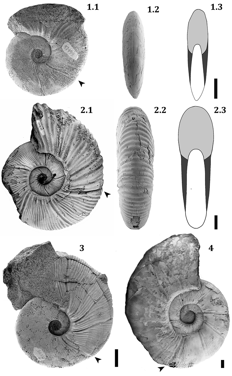
FIGURE 4. Descriptive terminology used for morphological parameters with a 30° step-width grid spanned over the median plane of a specimen of M. seymourianus to illustrate the procedure of data acquisition: 1. Longitudinal section. 2. Cross-section. Abbreviations: ah, aperture height; dm, diameter; uw, umbilical width; wh, whorl height; ww, whorl width. Scale bar = 10 mm.
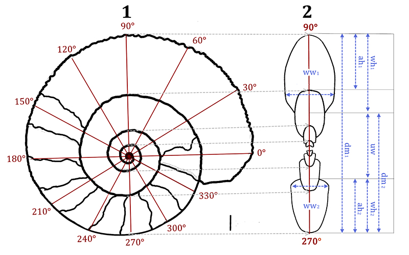
FIGURE 5. Theoretical Area Estimate (TAE) in whorl cross sections of: 1. M. seymourianus and 2. M. densicostatus.
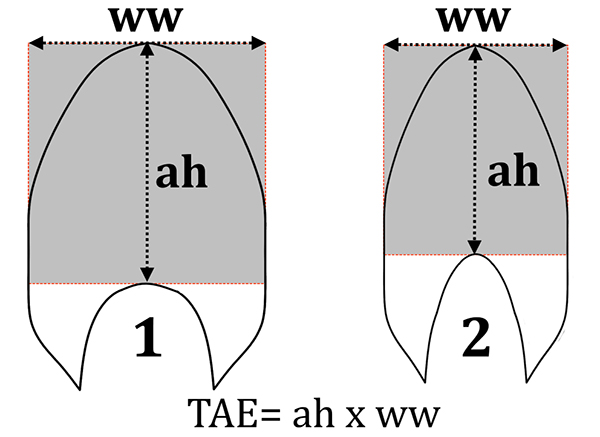
FIGURE 6. Linear plots of ontogenetic trajectories for each parameter against the shell diameter from Maorites seymourianus. 1: Aperture height. 2: Whorl height. 3: Whorl width. 4: Umbilical width. 5: Conch width index. 6: Whorl width index. 7: Umbilical width index. 8: Whorl expansion rate. The lines represent the statistical models in Table 1. P: Perlatum stage (black bars), G: Gibbosum stage (grey bars).
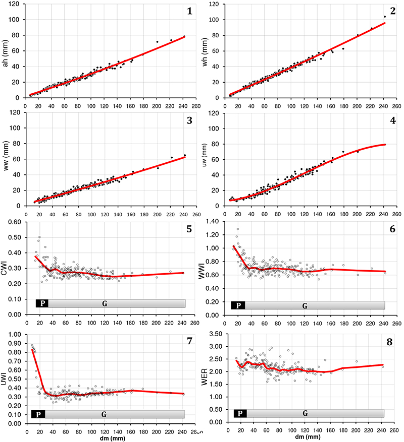
FIGURE 7. Linear plots of ontogenetic trajectories for each parameter against the shell diameter from Maorites densicostatus. 1: Aperture height. 2: Whorl height. 3: Whorl width. 4: Umbilical width. 5: Conch width index. 6: Whorl width index. 7: Umbilical width index. 8: Whorl expansion rate. The lines represent the statistical models summarized in Table 1. P: Perlatum stage (black bars), G: Gibbosum stage (grey bars).
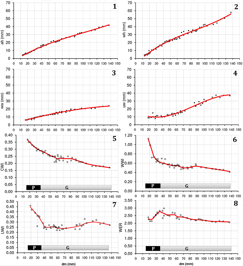
FIGURE 8. 3D models of Maorites seymourianus exhibiting the data lost during the reconstruction process. 1. M. seymourianus (CPBA-16847) in lateral view; 1.1: Specimen, 1.2: 3D model of the conch with four chambers, 1.3: 3D model of the conch, showing the position of four chambers,1.4: 3D models from the reconstructed chambers. 2. M. seymourianus (CPBA-16830); 2.1: 3D models of the conch and early chambers, 2.2: 3D models of the chambers showing the increase in suture complexity; note the first chambers are noticeably spaced (see text). 3: M. seymourianus (CPBA-16814) in lateral view. 3.1: Specimen, 3.2: 3D model of the conch, note the decrease of ornamentation in the model compared to the fossil specimen. Scale bars = 10 mm.
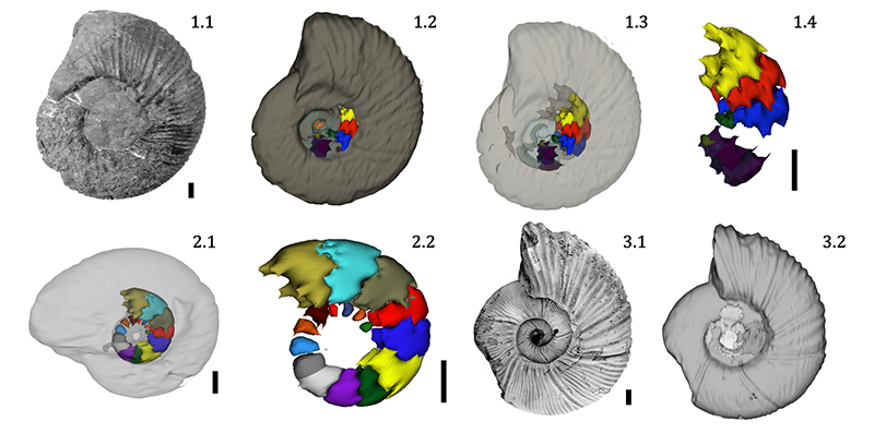
FIGURE 9. Comparison of ontogenetic trajectory models for each parameter against the shell diameter in the studied species, based on LOWESS models; dotted-lines indicate the limits of the 95% confidence band. Grey: Maorites seymourianus. Black: M. densicostatus. 1: Aperture height. 2. Whorl height. 3: Whorl width. 4: Conch width index. 5: Whorl width index. 6: Umbilical width index. 7: Whorl expansion rate. 8: Theoretical area estimate.
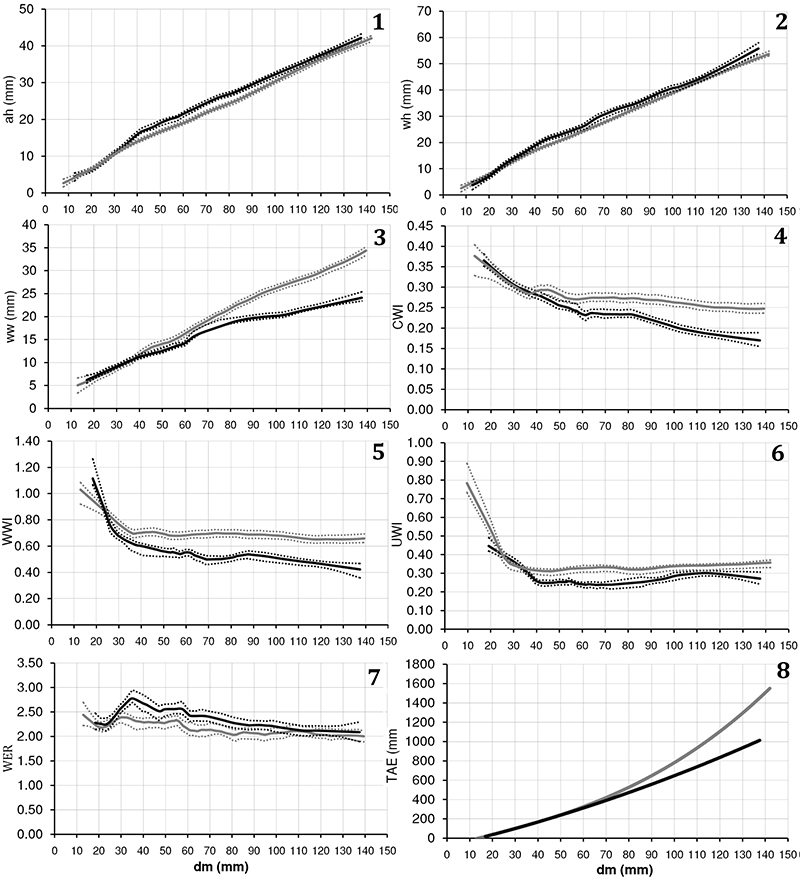
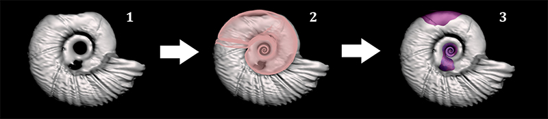
FIGURE 10. Three-dimensional reconstruction of a poorly preserved M. seymourianus conch. 1. 3D model of the shell derived from the computed tomography. 2. 3D model with the reconstructed section based on a mathematical model (Erlich et al. 2016). 3. 3D model and mathematical model fused in a complete shell.