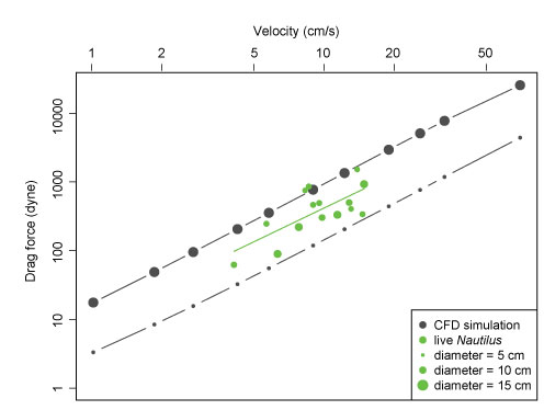
FIGURE 1. An outline of the workflow from model creation to completed simulation. Boxes are colored based on the general process they are included in: Case generation (blue), Mesh generation (purple), and numerical set-up (green). Two tracks are shown for case generation: one in which a model is created in blender from measurement data (below the dotted line) and the other where the model is created using a Structure from Motion technique such as laser scanning or photogrammetry (above the dotted line). Software used in each process is noted in “()” outside its respective step.
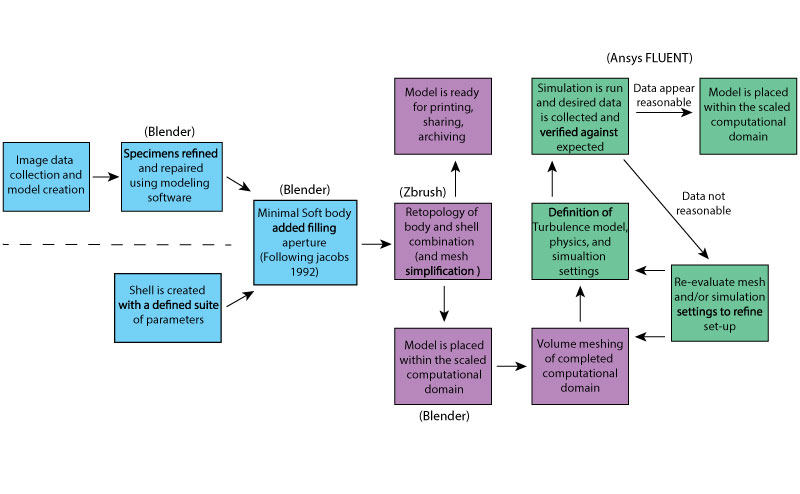
FIGURE 2. All of the shells employed in this study plotted in Westermann morphospace. The 3D models used for each member are shown to the right of the name/designation in the legend. Cardioceras, Oppelia, and Sphenodiscus are based on the shells employed in Jacobs (1992), Nautilus pompelius was created using laser scans and scaled to two different sizes (life-size [approx. 14.5 cm] and 5 cm diameter), and all other shells were created to match basic Westermann morphotypes (Westermann, 1996; Ritterbush and Bottjer, 2012).
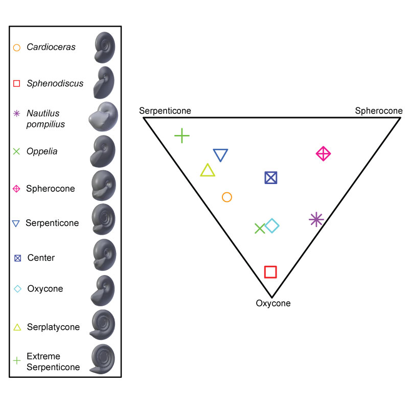
FIGURE 3. An illustration of the computational domain of the simulation. The model target (an ammonoid in this case) is shown as a circle. Each arrow indicates a distance from the shell to a target face of the computational domain. These arrows represent the straight-line distance between the nearest edge of the shell (not the shell's midpoint) and the corresponding wall as per the methods of Shiino, Kuwazuru, and Yoshikawa (2009). Dimensions in the figured example correspond to those of Scheme 3 (see Table 1).
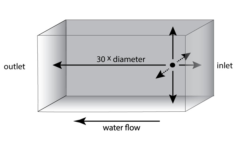
FIGURE 4. Hemisphere simulation data plotted as velocity versus % difference from the literature baseline (Blevins 1984). Velocities shown are within a range in which the drag coefficient of a hemisphere is relatively stable around a value of 1.17 (Blevins, 1984). The drag values used to derive this plot are given in Appendix 3.
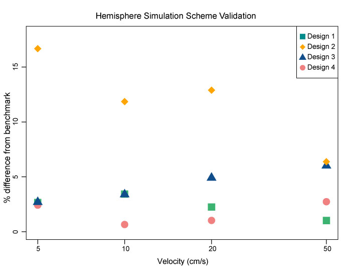
FIGURE 5. Coefficient of drag results from Scheme 1 (green) and Scheme 3 (blue) plotted against Re compared against the data from Jacobs (1992; black). Comparisons shown are for Sphenodiscus (left) and Oppelia (right).
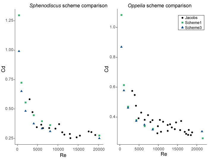
FIGURE 6. Examples of shape approximation errors resulting from the assembly meshing method. A) The surface expression of the Sphenodiscus shell that uses the tetrahedral meshing. B) The surface expression of the Sphenodiscus model that uses Assembly meshing. C) A cross-section through a hemisphere that uses the tetrahedral method. D) The same hemisphere cross-section using assembly meshing. In both B and C there is deformation and asymmetry in how the surface of the geometry is expressed leading to increased solution inaccuracy.
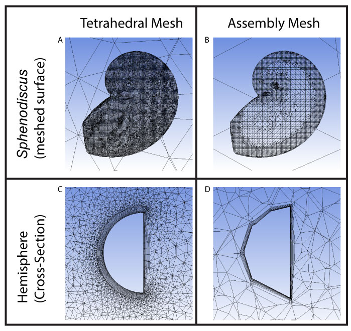
FIGURE 7. Plot of drag force versus velocity for each of the 10 different morphotypes used in this study. Only shells that had a uniform diameter of approx. 5 cm from aperture to venter are shown.
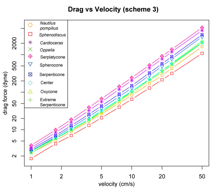
FIGURE 8. Plot of the coefficient of drag versus Reynolds number for each of the 10 morphotypes in this study. Drag coefficient and Reynolds number were calculated following the equations of Jacobs (1992). Only shells that had a uniform diameter of approx. 5 cm from aperture to venter are shown.
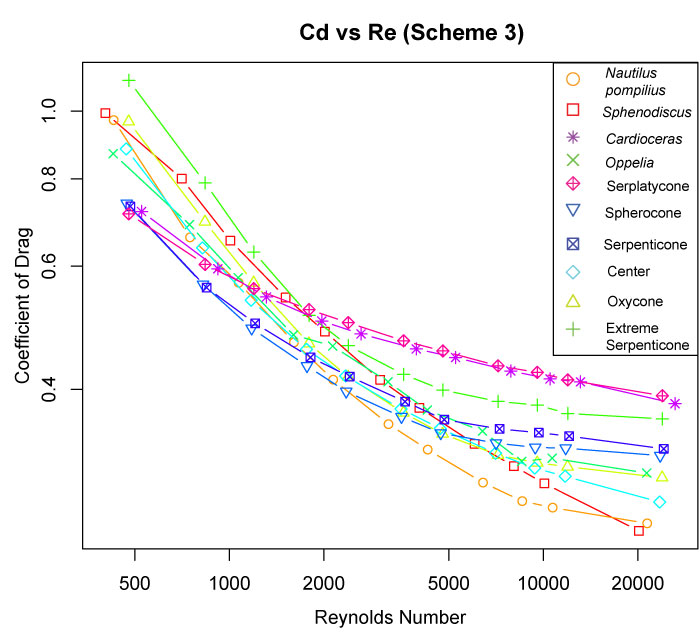
FIGURE 9. Water velocity around the Sphenodiscus shell at inlet velocities of 15 cm/s (A) and 5 cm/s (B). Areas of slow water velocity caused by viscous interactions are larger to the sides and immediately behind the shell at the lower velocity because water is less readily shed.
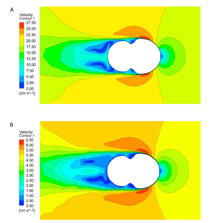
FIGURE 10. Comparison of the drag force at two different velocities (5 and 15 cm/s; Dotted and solid trendlines, respectively) across four different shell shapes. Shells represented (from left to right) include: Sphenodiscus, Cardioceras, Serpenticone, and Extreme Serpenticone). All four shells have 20-22% thickness ratio, and therefore plot along the left flank of Westermann Morphospace (see Figure 2). Umbilical exposure is a significant predictor of drag at both velocities but the components of the relationship change: a linear model of drag as a function of umbilical exposure yields an R2 value of 0.9987 for simulations at 15 cm/s (p value = 0.0007); a linear model of drag as a function of the natural log of umbilical exposure yields an R2 value of 0.9991 for simulations at 5 cm/s (p value = 0.0004; via R, R Core Development Team, 2019)
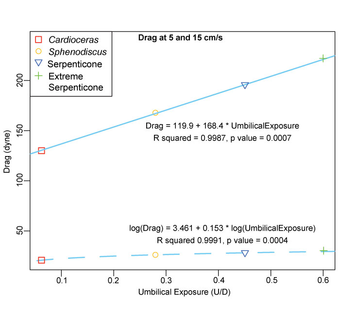
FIGURE 11. Plots of pressure overlain with water velocity vectors for the Serpenticone and Oxycone shells at both 15 cm/s (A) and 5 cm/s (B) inlet velocities. At 15 cm/s the flow around the Serpenticone shell is more chaotic and there is a buildup of pressure at around the trailing coils compared to the Oxycone shell. This difference mostly disappears at 5 cm/s.
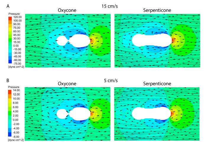
FIGURE 12. Simulated Nautilus data plotted alongside live Nautilus behavior data from Niel and Askew (2018).