FIGURE 1. Location map of Béon 1 locality, Montréal-du-Gers (MN4; mid-Orleanian, late early Miocene, south western France). The locality of Béon 1 is located (red circle) on the map of France (upper left corner) and on the zoom of south western France. Main cities (grey circles; bold) and rivers are indicated on the zoomed map. Dashed line represents the Spain-France frontier. Modified from Antoine and Duranthon (1997).
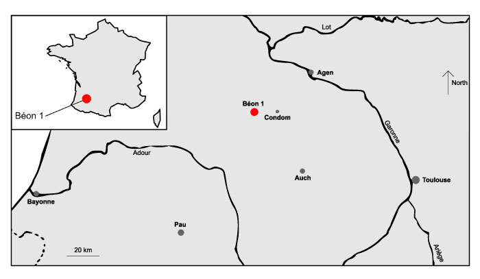
FIGURE 2. Localization of the microwear facets on rhinocerotid molars. Position of the two microwear facets (grinding and shearing) on the second upper molar (left) and second lower molar (right). Both facets are sampled on the same enamel band with (grinding) or without (shearing) Hunter-Schreger bands (HSB). Modified after Hullot et al. (2019).
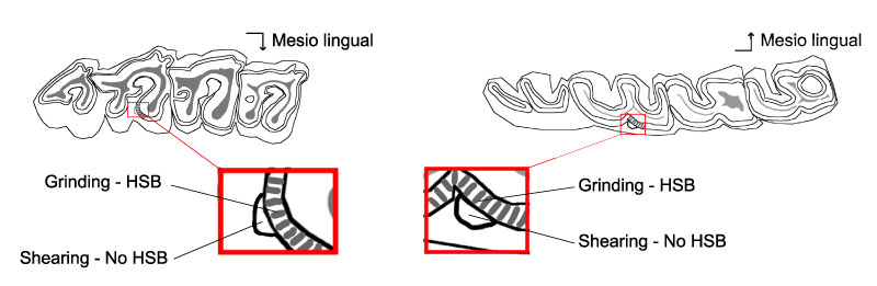
FIGURE 3. Principle of mesowear scoring with the main variables illustrated (occlusal relief and cusp shape) and examples on rhinocerotid teeth. A- Typically two parameters are studied in mesowear: cusp shape and occlusal relief. Cusp shape can be sharp, round or blunt, while occlusal relief is whether high or low. Illustration on the upper right M1 of the specimen MHNT.PAL.2004.0.58 (H. beonense). Examples of mesowear scores using the three methods tested in this study (ScoreA, ScoreB, Ruler) are provided on the paracone of the following specimens: B- Right D4 of MHNT.PAL.2015.0.1204 (G2 685; Pl. mirallesi), C- Left M1 and M2 MHNT.PAL.2015.0.277 (Pr. douvillei), D- Left D4 of MHNT.PAL.2015.0.1204 (Béon F2 193; Pl. mirallesi), E- Left D3 and D4 of MHNT.PAL.2015.0.2796 (Pr. douvillei). ScoreA: mesowear score based on Winkler and Kaiser (2011); B- ScoreB: mesowear score adapted from Fortelius and Solounias (2000); C- Ruler: mesowear score based on Mihlbachler et al. (2011)
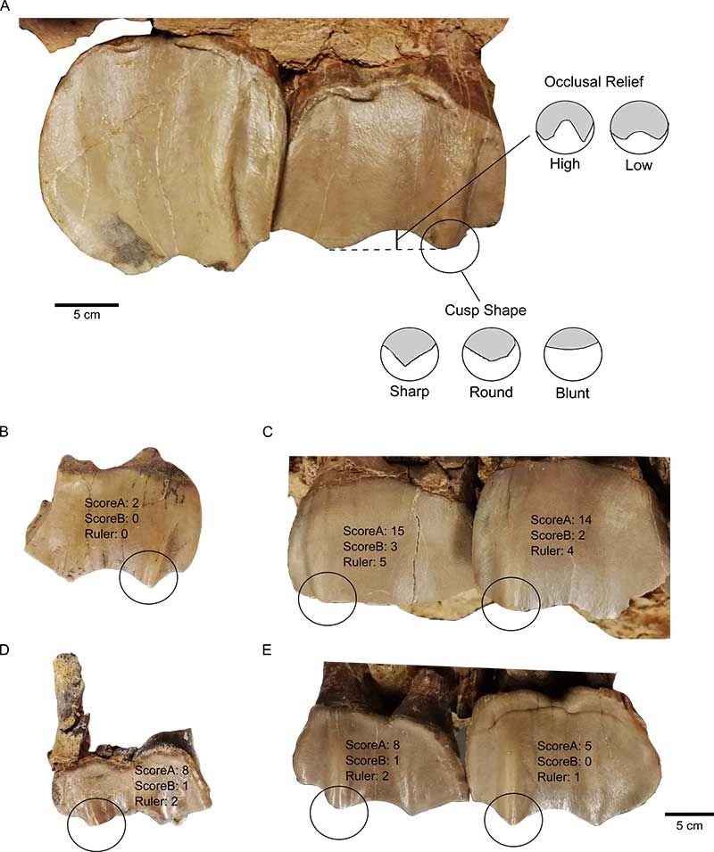
FIGURE 4. The three different types of hypoplasia considered in this study and the associated measurements. A- Lingual view of right M2 of the specimen MHNT.PAL.2004.0.58 (H. beonense) displaying three types of hypoplasia. B- Interpretative drawing of the photo in A illustrating the hypoplastic defects: a- pitted hypoplasia, b- linear enamel hypoplasia, and c- aplasia. C- Interpretative drawing of the photo in A illustrating the measurements: 1- distance between the base of the defect and the enamel-dentin junction, 2- width of the defect (when applicable).
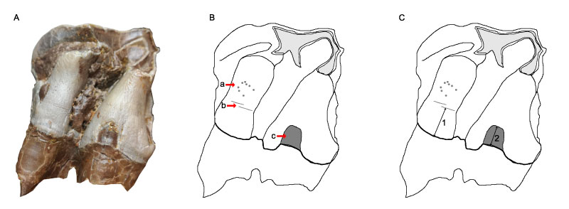
FIGURE 5. Comparison of the DMTA patterns by species, facet and preparation type. Upper graphs: hand-prepared specimens; lower graphs: sand-prepared specimens. Left graphs: grinding facet; right graphs: shearing facet. Boxplots of anisotropy and complexity were plotted along with the dotplots to facilitate graph interpretation.
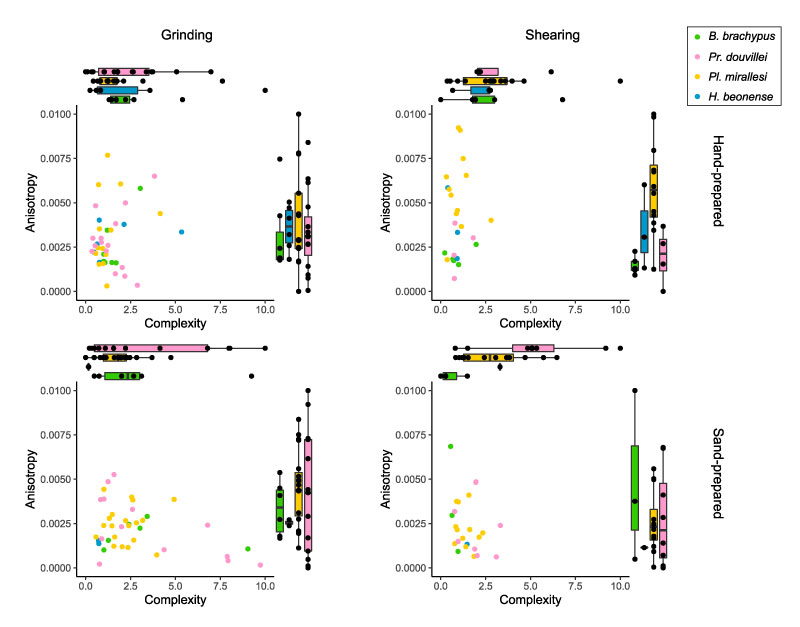
FIGURE 6. Comparison of hand- and sand-prepared DMTA surfaces (200x200 µm) by species. Topography and black and white photosimulation of the following specimens:
B. brachypus - hand-prepared MHNT.PAL.2015.0.1262 right m3 (protoconid, shearing facet) and sand-prepared MHNT.PAL.2015.0.2830 left m2 (hypoconid, shearing facet); Pr. douvillei - hand prepared MHNT.PAL.2015.0.1228 left m3 (protoconid, grinding facet) and sand-prepared MHNT.PAL.2015.0.2758 left m2 ptc (protoconid, grinding facet); Pl. mirallesi - hand-prepared MHNT.PAL.2015.0.1196 left m2 ptc (protoconid, shearing facet) and sand-prepared MHNT.PAL.2015.0.2794 (2002 E2 30) left m1 (hypoconid, shearing facet); H. beonense - hand-prepared MHNT.PAL.2015.0.1140 left m1 (hypoconid, grinding facet) and sand-prepared MHNT.PAL.2015.0. 1136.1 right M3 (protocone, grinding facet).
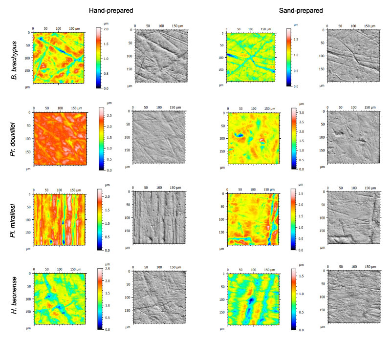
FIGURE 7. Percentages of specimens above anisotropy (epLsar > 0.005) or complexity (Asfc > 2) cutpoints by species, facet, and preparation type. Triangles: living rhinoceros’ species; circles: Béon 1 fossil rhinocerotids; size proportional to the number of specimens.
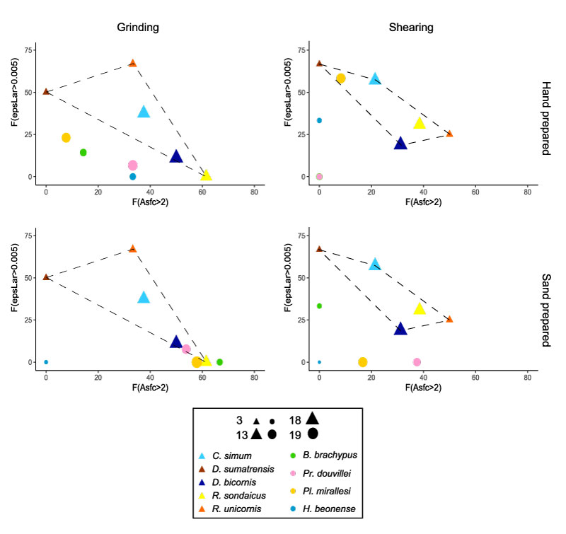
FIGURE 8. Barplots of mesowear scores on permanent teeth by method (ScoreA, ScoreB, Ruler) and by species. A- ScoreA: mesowear score based on Winkler and Kaiser (2011); B- ScoreB: mesowear score adapted from Fortelius and Solounias (2000); C- Ruler: mesowear score based on Mihlbachler et al. (2011). Only one tooth per specimen was considered.
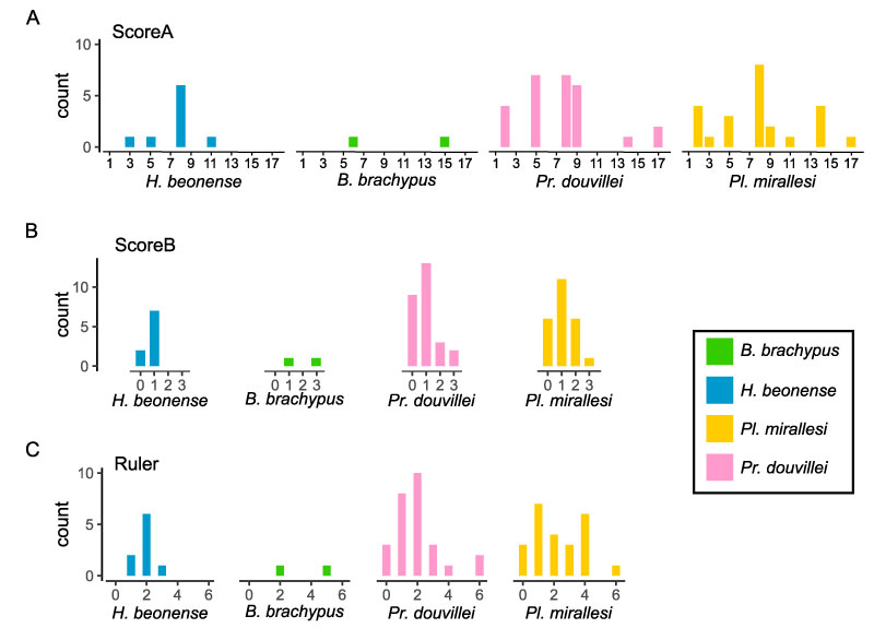
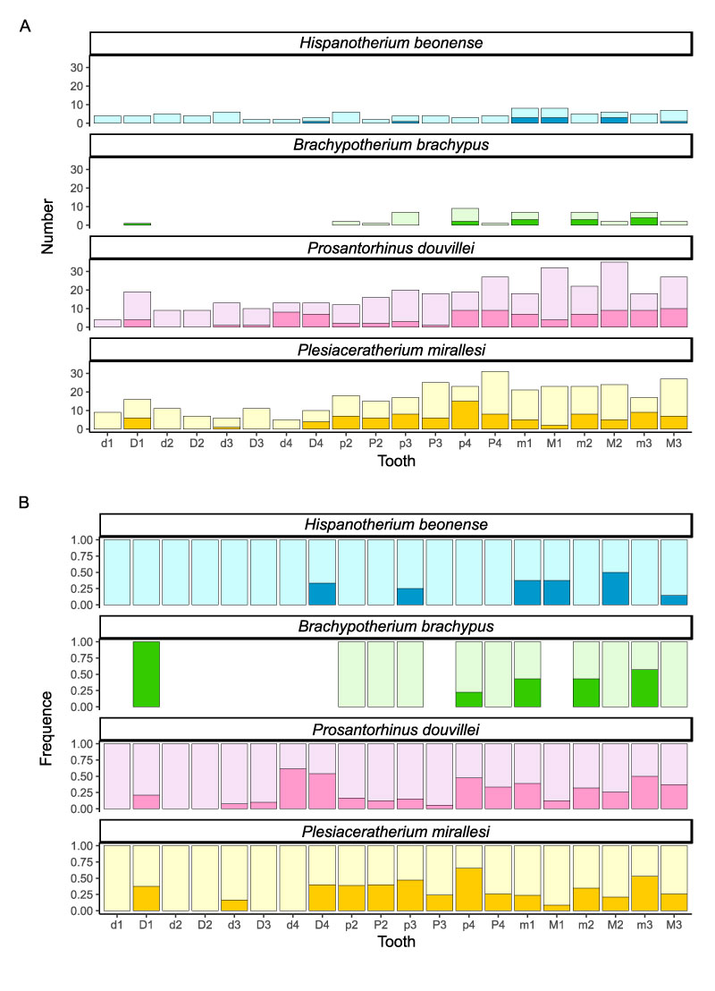
FIGURE 9. Prevalence of hypoplasia (all types) by species and tooth locus. A- Number of hypoplastic teeth (dark colors) compared to the number of healthy teeth (light colors). B- Frequency of hypoplastic teeth (dark colors) and healthy teeth (light colors). White stands for non-documented loci.