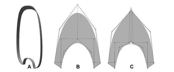
FIGURE 1. Summary of linear dimensions measured for the calculation of the Raupian parameters, and the shell diameter in a cross-section of an ammonoid. Some of these linear dimensions were adopted and modified by Korn (2010): whorl height (a = wh), whorl width (b = ww), maximum diameter (dm = d + e). Korn (2010) added some parameters to ammonoids such as the aperture height (f), the imprint zone (g), the umbilical width (h + c), and indices and rates related (see Korn 2010; Klug et al. 2015). (Modified from Raup, 1967)
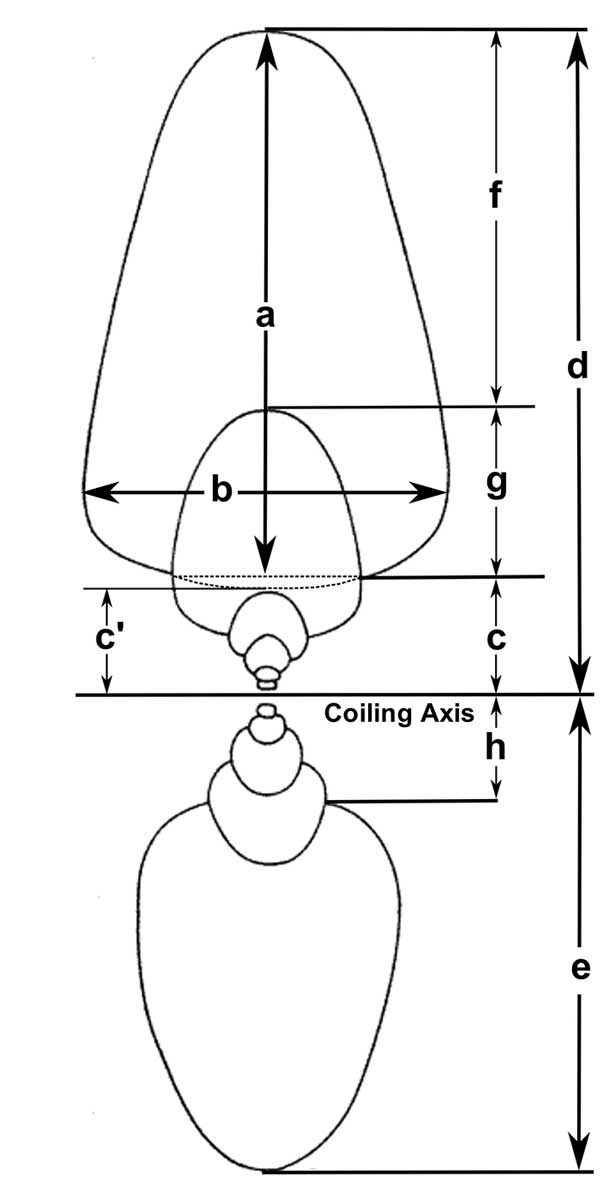
FIGURE 2. Catmull and Clark´s subdivision surface applied to a two-dimensional rectangular plane. A) Original plane. B) Result of one subdivision. C) Result of two subdivisions.
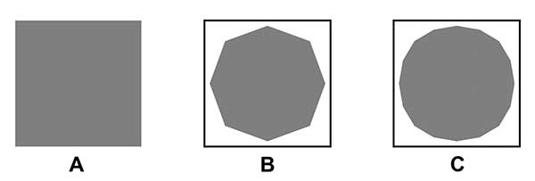
FIGURE 3. Virtual whorl cross-sections (grey surfaces) showing the 18 semilandmark configurations (black wireframes) used for this study (four subdivisions leves employed). A) Basic virtual model showing the zones defining the shape of a theoretical whorl cross-section in ammonoids. The horizontal length of the contact zone determines an acute or blunt transition between the dorsolateral zone and the imprint zone. B) Semilandmark model and virtual whorl cross-section for the ammonoid illustrated in Figure 1 at maximum diameter. C) Semilandmark model adapted to the heteromorph ammonoid Pedioceras multicostatum. In evolute ammonoids the contact and imprint zones are reduced, consequently, some of the semilandmarks share the same coordinates (the vertices are merged). D) Semilandmark model adapted to Nautilus pompilius. In nautilids the contact zone is trapezoidal following a rounded umbilicals wall.
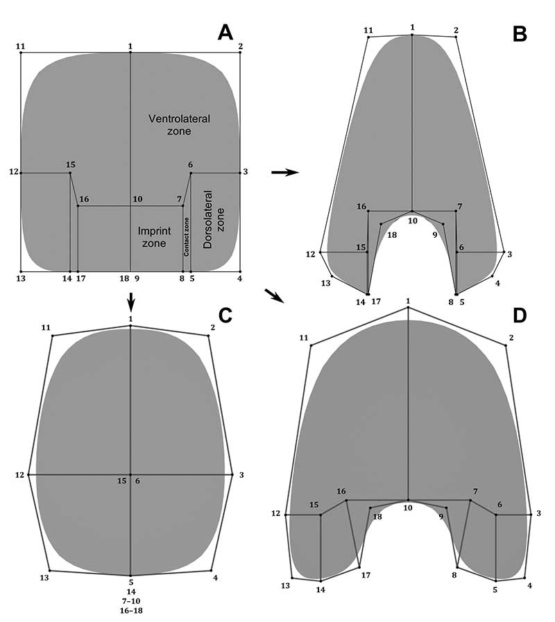
FIGURE 4. Covariation patterns derived from the standard model studied using a theoretical subrectangular whorl cross-section with the following parameters: aperture height (ah) = ¾, whorl width (ww) = 1, whorl height (wh) = 1. A) Semilandmark configuration showing the expected transformations from an arbitrary variation (± 0.1 units) in the whorl width, causing an expansion (red) or compression (blue). B) Graph bars showing the change in locations for each semilandmark in the horizontal x-axis from A. C) Semilandmark configuration showing the expected transformations from an arbitrary variation (± 0.1 units) in the aperture height and whorl height, causing an elongation (orange) or contraction (purple), and an increase (yellow) or decrease (green) in involution. D) Graph bars showing the change in locations for each semilandmark in the vertical y-axis from C. Note that a covariation pattern will be a combination of the x and y vectorial components (e.g., an expansion, elongation, and a decrease in involution).
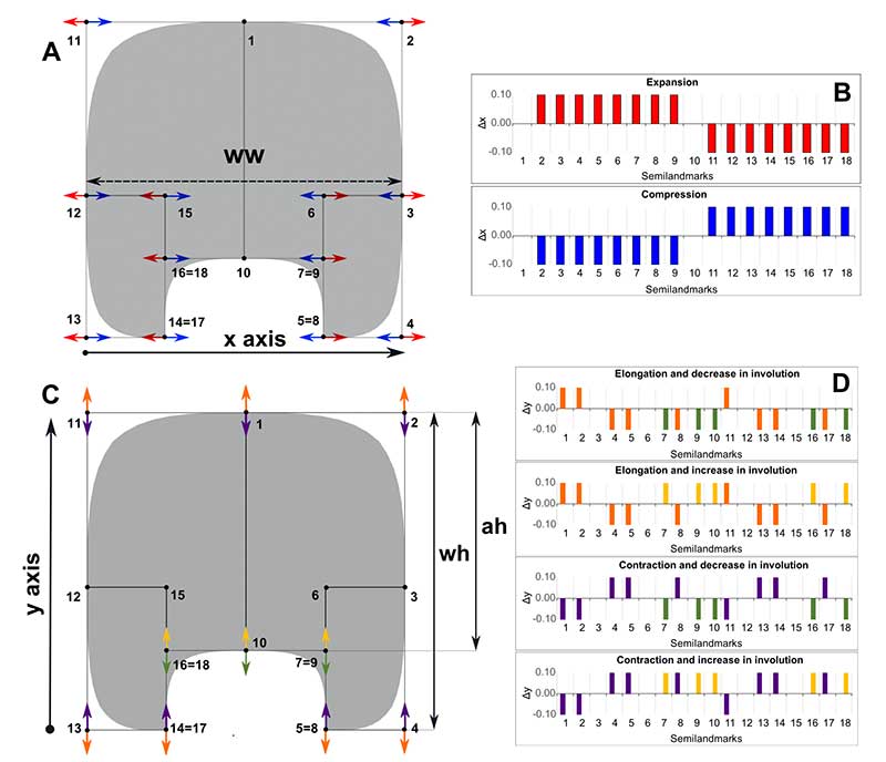
FIGURE 5. Transformations from negative to positive values in PC1. A) Semilandmark configuration at PC1=-0.4 showing the x (red) and y (blue) vectorial components towards PC1 positive values. B) Semilandmark configuration at PC1=0.4 obtained from the transformation of A. C). Graph bar illustrating the translations for each semilandmark in the x-axis for PC1. Empty bars illustrate the closest covariation pattern from Figure 4; in this case, transformations adjusted to an overall expansion of the whorl cross-section. D) Graph bar indicating the translations for each semilandmark in the y-axis for PC1. Empty bars illustrate the closest covariation pattern from Figure 4; in this case, a contraction with an increase in the involution degree. Note that the highest variation is observed on semilandmarks related to the imprint zone (5 to 9 and 14 to 18).
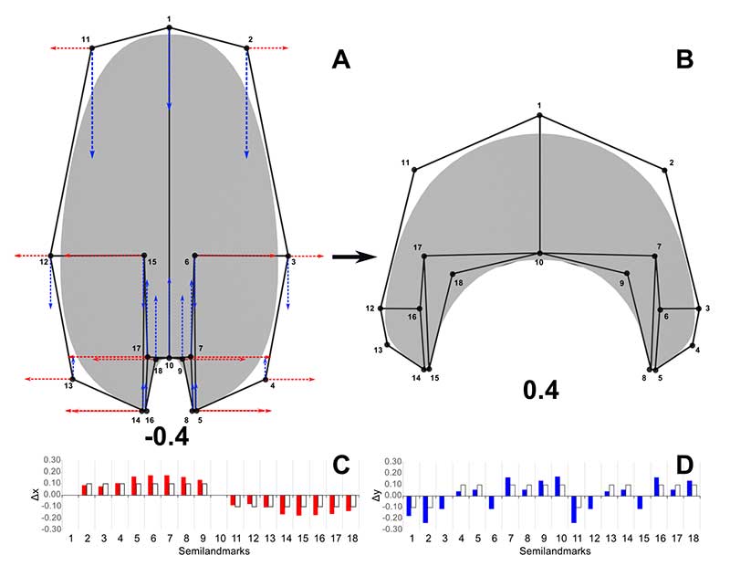
FIGURE 6. Transformations from negative to positive values in PC2. A) Semilandmark configuration at PC2=-0.3 showing the x (red) and y (blue) vectorial components towards PC2 positive values. B) Semilandmark configuration at PC2=0.3 obtained from the transformation in A. C). Translations for each semilandmark in the x-axis for PC2. Empty bars illustrate the closest covariation pattern from Figure 4; in this case, a localized compression in the peripheric landmarks (2 to 4 and 11 to 13). D) Translations for each semilandmark in the y-axis for PC2. Empty bars illustrate the closest covariation pattern from Figure 4; in this case, an elongation with an increase in the involution degree of the whorl cross-section.
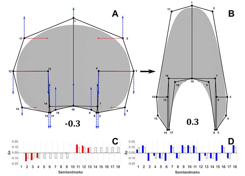
FIGURE 7. Transformations from negative to positive values in PC3. A) Semilandmark configuration at PC3=-0.3 showing the x (red) and y (blue) vectorial components towards PC3 positive values. B) Semilandmark configuration at PC3=0.3 obtained from the transformation in A. C). Translations for each semilandmark in the x-axis for PC3. Empty bars illustrate the closest covariation pattern from Figure 4; in this case, there is a weak adjustment to a compression of the whorl cross-section. D) Translations for each semilandmark in the y-axis for PC2. Empty bars illustrate the closest covariation pattern from Figure 4; in this case, a weak adjustment to a compression of the whorl cross-section. Note that most of the variation is in semilandmarks 3, 6, 12, and 15 that define the vertical location of the whorl width with respect to the whorl cross-section.
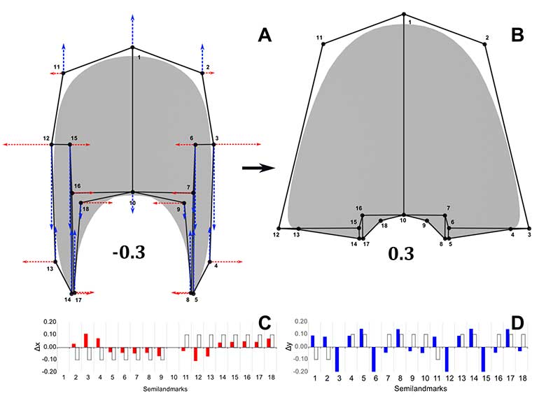
FIGURE 8. Morphospace formed by the first two PCs found in this study showing the location for each specimen in Table 3. The virtual whorl cross-sections of the PC-score values are illustrated below the axis. Combinations of these PC values are shown in the extremes of the morphospace. Evolute ammonoids are confined to a region to the left, this could be caused by a lack of subevolute specimens in the original sample.
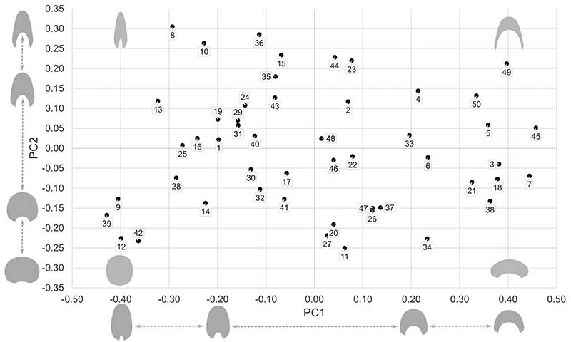
FIGURE 9. Morphospace formed by PC1 and PC3 from this study showing the location for each specimen in Table 3. The virtual whorl cross-sections for extreme values are illustrated below the axis of each PC.
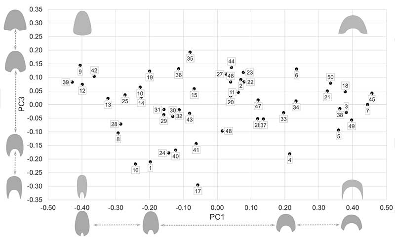
FIGURE 10. Morphologic variation in the diameter (dm) and the mean stratigraphic age range (MAR) illustrated through linear plots, showing the direct or inverse relationships of the variates. A) PC1 against the diameter (R² = 0.25, p = <0.05). B) PC1 against MAR (R² = 0.20, p = <0.05). C) PC2 against the diameter (R² = 0, p = 0.88). D) PC2, against MAR (R² = 0.22, p = <0.05).
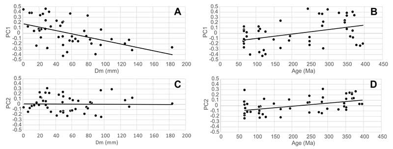
FIGURE 11. Morphological variation of the virtual whorl cross-section at different diameters in Proleymeriella schrammeni . Three ontogenetic stages can be distinguished. The first consists of a rapid morphological change at the beginning of the ontogeny with a predominance of PC1 transformations, this ontogenetic stage is followed by a short interval of morphological stasis. The third ontogenetic stage is likely related to maturity with a predominance of PC2 and PC3 transformations.
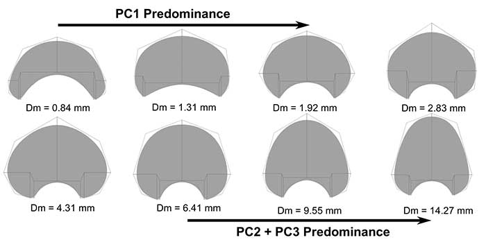
FIGURE 12. Examples of additional applications for the virtual modelling technique described in this study. A) Basic segment ready to generate a 3D virtual model for hydrodynamic and hydrostatic analyses based on the whorl cross-section of Deshayesites grandis (Bersac and Bert, 2012, figure 2). B-C) Semilandmark configuration and virtual whorl cross-section for the galeate ammonoid Paratornoceras lentiforme (Korn et al., 2020, figure 5A). B) Simplified virtual whorl cross-section based on the 18 semilandmarks model used in this study. C) Modified virtual whorl cross-section based on a 24 semilandmarks model adjusted to emphasize the sharp ventral region.