FIGURE 1. Summary of the morphometric and geometric morphometric (GM) models used in this work. A) Cross-section of an ammonoid showing the standard morphometric model to study the ammonoid conch morphology presented by Korn (2010) and Klug et al. (2015). Abbreviations: ah, aperture height; dm, diameter; iz, imprint zone; wh, whorl height, ww, whorl width. B-E) Geometric morphometric model to study the whorl shape presented in Morón-Alfonso et al. (2021). B) Basic virtual model (grey area) showing the corresponding configuration based on 18 semi-landmarks. C) GM model adapted to the specimen shown in A. D) GM model applied to the whorl of an evolute specimen. E) GM model applied to the whorl profile of an involute specimen (modified from Raup 1967).
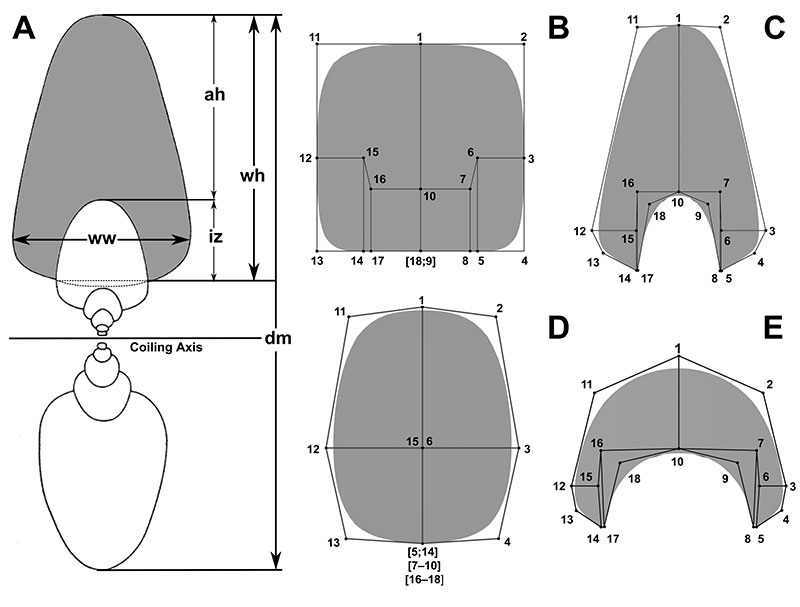
FIGURE 2. Workflow employed in this work. The squares identify the produced data, and the hexagons indicate the analyses and procedures.
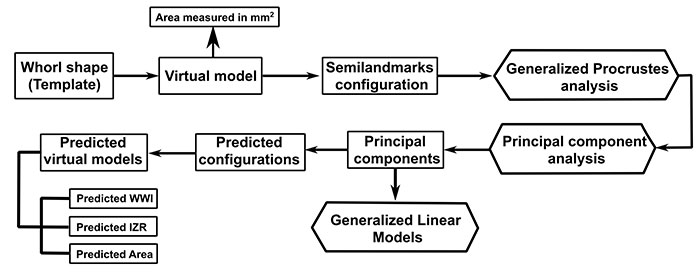
FIGURE 3. Density plot of the ammonoid genera through time. Occurrences of major extinction events are signalled as dashed lines, minor extinction events relevant to ammonoid diversity are illustrated as dotted lines based on Bambach et al. (2004).
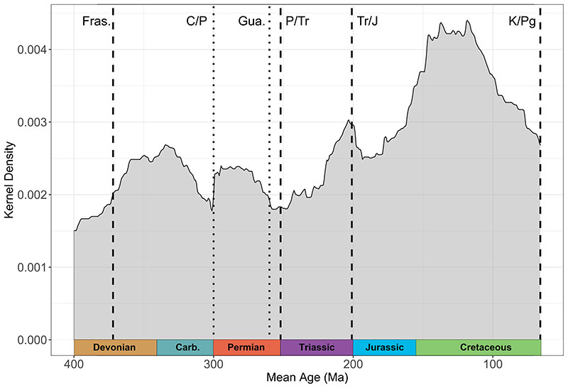
FIGURE 4. Paleolatitude of the original locality for each ammonoid specimen through time. Note the widespread distribution of the clade.
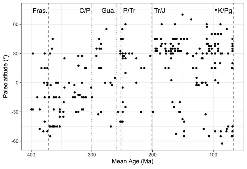
FIGURE 5. Major subclades (order level) within Ammonoida based on sutural/septal classification through time. Occurrences of major extinction events are signalled as dashed lines, minor extinction events relevant to ammonoid diversity are illustrated as dotted lines based on Bambach et al. (2004).
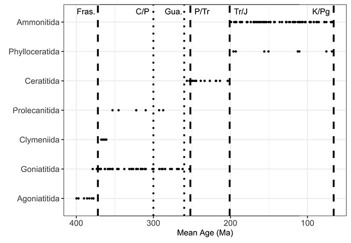
FIGURE 6. Boxplots for the first three principal components for the subtaxa used in this work. A) Subtaxa against PC1. B) Subtaxa against PC2. C) Subtaxa against PC3.
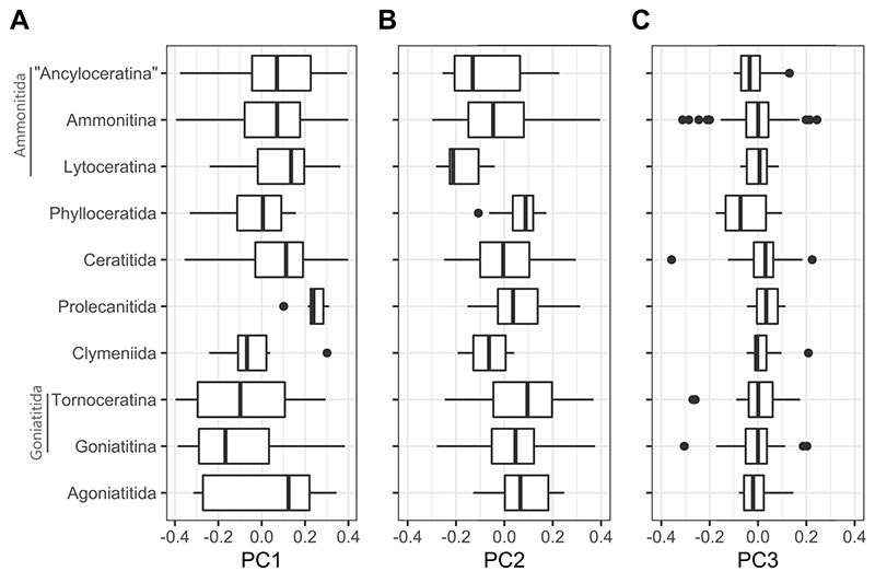
FIGURE 7. Morphospace for the WPS based on the first three principal components showing the density curves. A) Scatter plot for PC1 and PC2. B) Density heat map for PC1 and PC2. C) Scatter plot for PC1 and PC3. D) Density heat map for PC1 and PC3.
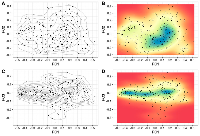
FIGURE 8. A) Backtransform morphospace for PC1 and PC2 showing the variations on the semilandmark configurations. B) Bivariate plots for the predicted configurations obtained from A for PC3score = 0.
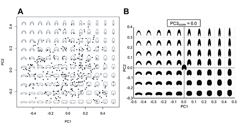
FIGURE 9. A) Backtransform morphospace for PC1 and PC3. B) Same as A but for PC2 and PC3.
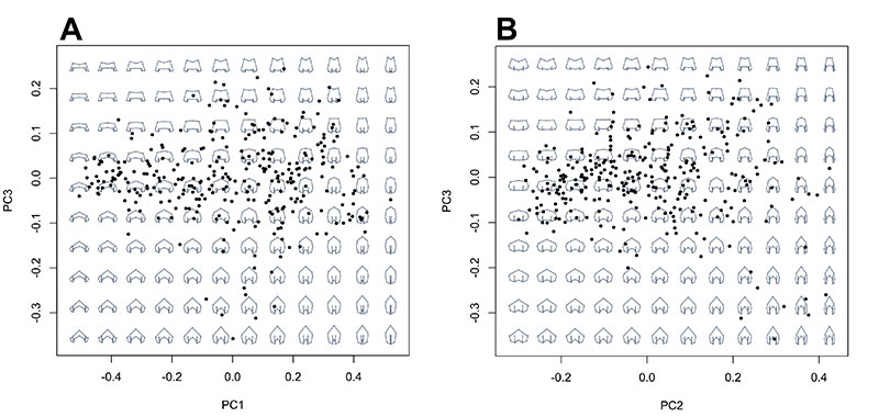
FIGURE 10. Bivariate plots illustrating the shape variation from the obtained morphospace for the first three principal components. Shadowed cells indicate the space that is occupied by the ammonoid genera.
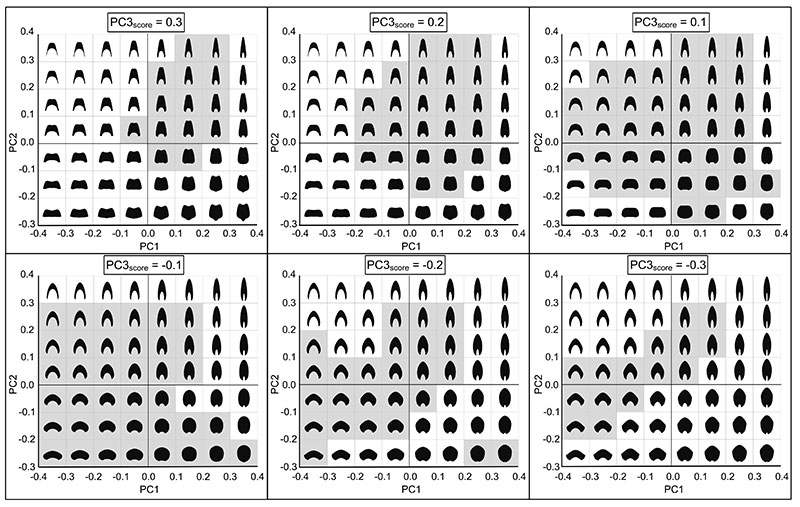
FIGURE 11. Predicted score PC1 values for the simple additive model 1 presented in Table 2 including the centroid size (CS), and the subtaxa, as predictors. Estimates with 95% of confidence. A) Predicted values for the centroid size (CS). B) Predicted values of PC1 for the selected subtaxa.
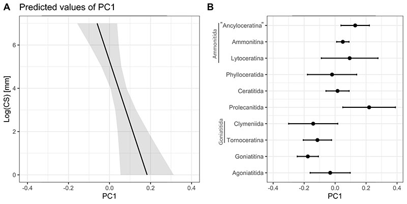
FIGURE 12. Variation of the measured area against different response variables. A) Relationship between the area and the diameter. B) Relationship between the area and the whorl height in mm. C). Relationship between the area and centroid size (CS). D) variation of the measured area for each of the selected subtaxa.
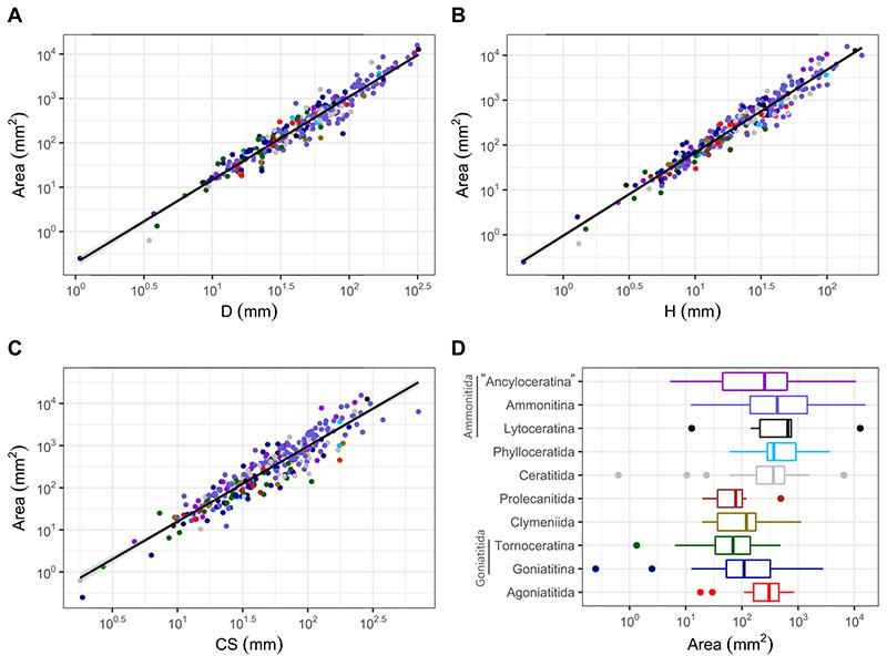
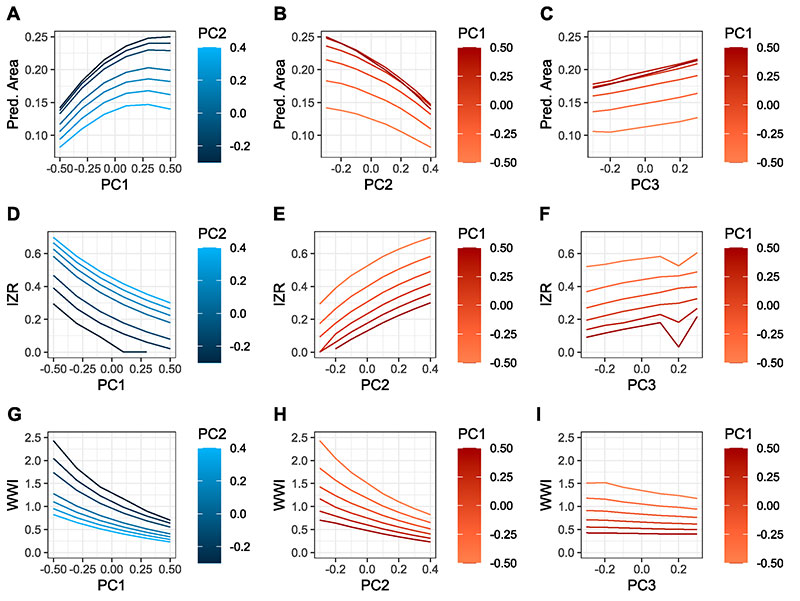
FIGURE 13. A-I) Variation of the predicted whorl area, the whorl width index (WWI=ww/wh), and the imprint zone rate (IZR=iz/wh) considering the first three PCs measured from the virtual models presented in Figure 10. The predicted area has no spatial units. A) Predicted area for PC1 at different PC2 values. Note PC1 has a local maximum depending on the score values of PC2 and PC3. B) Predicted area for PC2 at different PC1 values. C) Predicted area for PC3 at different PC1 values. D) Predicted WWI for PC1 at different PC2 values. E) Predicted WWI for PC2 at different PC1 values. F) Predicted WWI for PC3 at different PC1 values. Note that at low PC1 values changes for the WWI are not noticeable, and only at high PC1 values the changes become significant for PC3. G) Predicted IZR for PC1 at different PC2 values. H) Predicted IZR for PC2 at different PC1 values. I) Predicted IZR for PC3 at different PC1 values.