

APPENDIX 1.
List of localities and specimens.
Information is in the following order: full name of a locality, abbreviation in parentheses (bolded; abbreviation used in text and for all Figs and Tabs), collector and collecting year, geographic position, collection numbers. Abbreviations: f, female; m, male; PtU, sample (7) of the Pechora chromosomal race, 'Ulashevo;' SeF, sample (6) of the Serov race, 'Foothill' (ca. 300 m asl); SeH, sample (5) of the Serov race, 'Hill' (ca. 550 m asl); SeV, sample (8) of the Serov race, 'Valley' (ca. 180 m asl); ZIN, collection of the Zoological Institute of the Russian Academy of Sciences, St. Petersburg.
Sorex araneus
1. Artybash Village vicinity, Turochaksky District, Altay Republic, Russia (A1); Zaitsev, M.V., 12-13 August 1984; N 51.78, E 87.25: ZIN 73221 (f), ZIN 73237 (m) (n = 2).
2. Dan' Village vicinity, Kortkerossky District, Komi Republic, Russia (Da, Dan', ars); Kuprianova, I.F. and Bobretsov, A.V., July-August 1987-1988; N 61.38, E 51.80: ZIN 107851/654, /711, /1562, /1133, /1189, /1536 (n = 6).
3. Kurya [Kur'ya] Village vicinity, Krasnogorsky District, Udmurt Republic, Russia; Rodchenkova, E., 16 June 2009; N 57.70, E 52.01: ZIN 98446 (ZIN-TER-M-2082) (n = 1).
4. 'North Ural (tundra),' Russia; Vardonits (?), 3 August 1909; regional coord. ca. N 62.00, E 59.45: ZIN 140-1926 (n = 1).
5. Ser'ga River, Olenii Ruch'i Nature Reserve, Nizhneserginsky District, Sverdlovskaya Oblast', Russia (A2); Maksimova, E.G., June 2006; N 56.51, E 59.25: ZIN 96958, ZIN 96960 (n = 2).
6. Jani Peak of Ural. Mts. (Yanypupuner Ridge), Troitsko-Pechorsky District, Komi Republic, Russia (SeH); Kuprianova, I.F. and Bobretsov, A.V., July-August, 1995, 2001; N 62.08, E 59.08: ZIN 107832/77, /80, /134, /135, /171, /189, /190, 261, /264, /265, /283, /284, /288, /328, /329, /333, /334, /335, /372, /432, /435, /477, /511, /512, /513, /515, /559, /560, /562, /563, /625, /642, /643, /644, /669, /670, /671, /672, /673, /674, /771, /777, /788, /807, /811, /816, /818, /887, /923, /924, /926, /927, /929, /931, /932, /1015, /1036, /1044, /1045, /1046, /1061, /1066, /1072 (n = 63; 25 males/38 females).
7. Garevka Village vicinity, Troitsko-Pechorsky District, Komi Republic, Russia (SeF); Kuprianova, I.F. and Bobretsov, A.V., July-August, 2001-2002; N 61.05, E 58.27: ZIN 107831/686, /790, /791, /792, /890, /893, /1063, /1064, /1065, /1067, /1146, /1162, /1163, /1164, /1165, /1166, /1225, /1229, /1314, /1315, /1316, /1380, /1381, /1382, /1383, /1384, /1385, /1386, /1399, /1401, /1403, /1405, /1406, /1407, /1408, /1462, /1463, /1464, /1466, /1467, /1547, /1548, /1549, /1550, /1557, /1559, /1560, /1579, /1581, /1584, /1586, /2431, /2541, /2571, /2579, /2678, /2775, /2776, /2795, /2803, /2828, /2829, /2831, /2833, /2881, /2929, /2962, /2965, /2966, /2976, /2997, /2998, /2999, /3001, /3031 (n = 75; 38 males/37 females).
8. Ulashevo Village vicinity, Pechora District, Komi Republic, Russia (PtU, ars); Kuprianova, I.F. and Bobretsov, A.V., July-August, 1992; N 65.42, E 57.12: ZIN 107833/1001, /1002, /1007, /1009, /1011, /1012, /1017, /1018, /1019, /1021, /1022, /1023, /1024, /1026, /1027, /1030, /1032, /1034, /1037, /1042, /1046, /1048, /1049, /1053, /1055, /1057, /1061, /1062, /1070, /1073, /1076, /1078, /1079, /1080, /1081, /1082, /1093, /1095, /1096, /1101, /1102, /1105, /1113, /1120, /1122, /1127, /1142, /1145, 1148, /1149, /1152, /1165, /1173, /1174, /1181 (n = 55; 30 males/25 females).
9. Yaksha Village vicinity, Troitsko-Pechorsky District, Komi Republic, Russia (SeV); Kuprianova, I.F. and Bobretsov, A.V., July-August, 2001-2002; N 61.82, E 56.84: ZIN 107830/307, /314, /328, /329, /333, /334, /337, /338, /366, /367, /368, /395, /403, /404, /412, /414, /415, /420, /422, /434, /435, /461, /476, /478, /482, /484, /487, /488, /526, /533, /534, /545, /546, /558, /560, /562, /574, /615, /616, /1101, /1113, /1114, /1115, /1128, /1129, /1130, /1132, /1142, /1151, /1157, /1162, /1184, /1185, /1189, /1193, /1276, /1281, /1282, /1308 (n = 59; 27 males/32 females).
Sorex tundrensis--within the S. araneus geographic range:
10. 'Akademgorodok' (Novosibirsk Academic Campus), Sovetsky District of the city of Novosibirsk, Russia (T1); Drozdova, Yu.V., 19 October 1971; N 54.83, E 83.10: ZIN 67675 (f) (n = 1).
11. Dan' Village vicinity, Kortkerossky District, Komi Republic, Russia (Da, Dan', tdr); Kuprianova, I.F. and Bobretsov, A.V., July-August 1987-1988; N 61.38, E 51.80: ZIN 107852/727, /957*, /1089, /1129, /1182*, /1221* (n = 6).
* -- species determination by Dr. Nikolay E. Dokuchaev (re-determination S. araneus to S. tundrensis); other specimens of Dan' sample determined by Dr. Leonid L. Voyta during the material preparation for study of Shchipanov et al. (2014).
12. Kokorja Village vicinity, Kosh-Agachsky District, Altay Republic, Russia (T2); Abramov, A.V., Lopatina, N.V. and Platonov, V.V., 3-8 September 2013; N 50.17, E 89.27: ZIN 101862 (f), 101863 (m), 101864 (m), 101865 (m), 101866 (m) (n = 5).
13. Kyrlyk Village vicinity, Kosh-Agachsky District, Altay Republic, Russia (T3); Abramov, A.V., Lopatina, N.V. and Platonov, V.V., 21 September 2013; N 50.85, E 84.97: ZIN 101876 (m), 101877 (f) (n = 2).
14. Ramen'e Village vicinity, Velsky District, Arkhangelskaya Oblast', Russia (Ra); Kuprianova, I.F. and Bobretsov, A.V., July-August 1980-1981; N 61.00, E 42.00: ZIN 107850/1189 (n = 1).
15. Tashanta Village vicinity, Ust-Kansky District, Altay Republic, Russia (T4); Abramov, A.V., Lopatina, N.V. and Platonov, V.V., 29-31 August 2013; N 49.21, E 89.51: ZIN 101858, 101859 (m), 101860 (m), 101861 (f) (n = 4).
16. Ulashevo Village vicinity, Pechora District, Komi Republic, Russia (PtU, tdr); Kuprianova, I.F. and Bobretsov, A.V., July-August, 1992; N 65.42, E 57.12: ZIN 107849/1063 (male, n = 1).
>-- out of the S. araneus geographic range:
17. Kolyma River (upper part), Magadanskaya Oblast', Russia (T5); Okhotina, M.V., 4-7 August 1969; regional coord. ca. N 62.28, E 147.71: ZIN 90452 (m), ZIN 90453 (m) (n = 2).
18. Moneron Island, Sachalinskaya Oblast', Russia (T6); Okhotina, M.V., 7-8 August 1976; N 46.23, E 141.21: ZIN 91534 (f), ZIN 91535 (m) (n = 2).
19. Razdolno'e Village vicinity, Nadezhdinsky District, Primorsky Kray, Russia (T7); Okhotina, M.V., 26-30 September 1976; N 43.53, E 131.88: ZIN 90321 (m), ZIN 90328 (m) (n = 2).
20. 'Yakutia,' Megino-Kangalassky District, Republic of Sakha (Yakutia), Russia; Larionov, L.D., Summer 1952; regional coord. ca. N 61.96, E 129.91: ZIN 43608 (n = 1).
APPENDIX 2.
List of fossil specimens.
Information is in the following order: full name of a locality, abbreviation in parentheses (bolded; abbreviation used in text and for all Figures and Tables), geographic location, collector and collecting year, collection numbers. Preliminar species identification by Dr. Evgeny P. Izvarin. Abbreviations: IPAE, collection of the Institute of Plant and Animal Ecology of the Ural Branch of the Russian Academy of Sciences, Yekaterinburg. mb (mandible) and m1 (first lower molar) in square brackets mark availability of landmark data sets (see Material.section).
1. Cheremukhovo-1 Cave (Cher1): Rock Massif Chertovo Gorodishche on the right bank of the Sos'va River, North Ural (N 57.21, E 31.27); collector Dr. Tatyana V. Strukova (Strukova et al., 2006):
(Cher1/4) -- quadrat D/3, layer 4: Sorex araneus: IPAE C4/21 [mb, m1] (n = 1).
(Cher1/4-5) -- quadrat D/3, layers 4-5: Sorex araneus: IPAE C4-5/13 [mb, m1], C4-5/23 [mb, m1] (n = 2).
(Cher1/5) -- quadrat D/3, layer 5, horizon 45-65 см (5673±94 cal BP): Sorex araneus: IPAE C5/14 [mb, m1], C5/15 [m1], C5/24 [mb, m1] (n = 3).
Notes: in a numbers 'C4-C5' are layers; '/N' is particular attribute; based on the spatial relation of the layers, we, conventionally, consider Cher1/4 and Cher1/4-5 same aged to Cher1/5 (Figure 2: Cher1/5).
2. Dyrovatyi Kamen' Grot (DKS, DKS3): Ser'ga River, Middle Ural (N 56.51, E 59.25); collector Prof. Nikolay G. Smirnov, 1992 (Smirnov, 1993; Ulitko, 2006):
(DKS3/11) -- layer 3, quadrat E/8, horizon 11 (10557±234 cal BP):
Sorex araneus: IPAE DK01 [mb, m1], DK25 [mb, m1], DK26 [mb, m1], DK28 [mb, m1], DK29 [mb, m1], DK30 [mb, m1], DK31 [mb, m1] (n = 7).
Sorex cf. araneus: IPAE DK05 [m1] (n = 1).
Sorex tundrensis: IPAE DK08 [mb, m1], DK09 [mb, m1], DK10 [m1], DK32 [mb, m1], DK33 [mb, m1], DK34 [mb, m1], DK35 [mb, m1], DK36 [mb, m1], DK37 [mb, m1] (n = 9).
3. Sim III Cave (Sim3): Sim River, South Ural (N 54.90, E 57.78); collector Prof. Nikolay G. Smirnov (Smirnov et al.,1990):
(Sim3/2а) -- layer 2a (lens within 2b layer), depth 5-15 см (2940±258 cal BP):
Sorex araneus: IPAE S16 [mb, m1], S17 [mb, m1], S38 [mb, m1], S39 [mb, m1], S40 [mb, m1], S41 [mb, m1] (n = 6).
Sorex tundrensis: IPAE S18 [mb, m1], S19 [mb, m1] (n = 2); re-identified after the PCA analysis (see the main text).
TABLE A2-1. Radiocarbon dates for analyzed fossil samples, included calibrated dates from Fadeeva (2016). The calibrated dates (cal) have been obtained through the intCal20 Curve (Reimer et al., 2020). Abbreviations: B. Makh., Bolshaya Makhnevskaya Cave (horizon 140-147 cm); GIN, Geological Institute of the Russian Academy of Sciences, Moscow; SEVIN, A.N. Severtsov Institute of Ecology and Evolution of the Russian Academy of Sciences, Moscow; Koziy S., Koziy Stone Rock (horizon 135-145 cm); Rasik/B21, Rasik Grot (layer 21); Rasik/B27, Rasik Grot (layer 27).
| Current analyses data | ||||
| Sim3 | Cher1 | DKS3 | ||
| Layer/Horizon | 2a | 5 | 3 | |
| Source | small mammals | small mammals | small mammals | |
| Lab No | SEVIN 724 | SOAN 5137 | SEVIN 1075 | |
| 14C±σ | 2790±207 | 4930±75 | 9327±158 | |
| cal: Mean±σ | 2940±258 | 5673±94 | 10557±237 | |
| cal interval: from (95.4%) to (95.4%) | 3396-2366 | 5897-5483 | 11093-10223 | |
| Data from Fadeeva (2016) | ||||
| B. Makh. | Koziy S. | Rasik/B21 | Rasik/B27 | |
| Layer/Horizon | 140-147 cm | 135-145 cm | B21 | B27 |
| Source | rodents | rodents | rodents | rodents |
| Lab No | SEVIN 1385 | SEVIN 1332 | GIN 10569 | GIN 10567 |
| 14C±σ | 3628±86 | 9467±252 | 12680±180 | 13330±120 |
| cal: Mean±σ | 3951±125 | 10786±353 | 15008±355 | 16035±178 |
| cal interval: from (95.4%) to (95.4%) | 4226-3696 | 11611-10161 | 15634-14279 | 16379-15680 |
REFERENCES
Reimer, P.J., Austin, W.E.N., Bard, E., Bayliss, A., Blackwell, P.G., Ramsey, C.B., Butzin, M., Cheng, H., Edwards, R.L., Friedrich, M., Grootes, P.M., Guilderson, T.P., Hajdas, I., Heaton, T.J., Hogg, A,G., Hughen, K.A., Kromer, B., Manning, S.W., Muscheler, R., Palmer, J.G., Pearson, C., van der Plicht, J., Reimer, R.W., Richards, D.A., Scott, E.M., Southon, J.R., Turney, C.S.M., Wacker, L., Adolphi, F., Büntgen, U., Capano, M., Fahrni, S.M., Fogtmann-Schulz, A., Friedrich, R., Köhler, P., Kudsk, S., Miyake, F., Olsen, J., Reinig, F., Sakamoto, M., Sookdeo, A. and Talamo, S. 2020. The INTCAL20 Northern Hemisphere radiocarbon age calibration curve (0-55 cal kbp). Radiocarbon, 62:725-757.
Smirnov, N.G. 1993. Small mammals of the Middle Urals in Late Pleistocene/Holocene. Nauka, Ekaterinburg. (In Russian)
Smirnov, N.G., Bolshakov, V.N., Kosintsev, P.A., Panova, N.K., Korobeinikov, Yu.I., Olshvang, V.N., Erokhin, N.G. and Bykova, G.V. 1990. Istoricheskaya ekologiya zhivotnikh gor Yuzhnogo Urala. UrO AN SSSR, Sverdlovsk (In Russian)
Strukova, T.V., Bachura, O.P., Borodin, A.V. and Stefanovskii, V.V. 2006. Mammal fauna first found in alluvial-speleogenic formations of the Late Neopleistocene and Holocene, Northern Urals, locality Cheremukhovo-1. Stratigraphy and Geological Correlation, 14:91-101.
Ulitko, A.I. 2006. Golotsenovye mlekopitaushchie iz karstovykh polostei Srednego Urala, p. 243-247. In Savinetcky, A.B. (ed.), Dinamika sovremennykh ekosistem v golotsene. Materialy Rossiyskoy nauchnoy konferentsii. Izdatelstvo KMK, Moskwa (In Russian)
APPENDIX 3.
Support information for geometric morphometric analysis and landmark description.
FIGURE A3-1. Landmarks position on the medial surface of the dentary in relation to the teeth in recent materials and the alveoli edges in fossils. The image admits a similar position of the landmarks with and without teeth. For an unambiguous definition of the landmarks position is required a marking the alveoli edge before a photo acquisition.
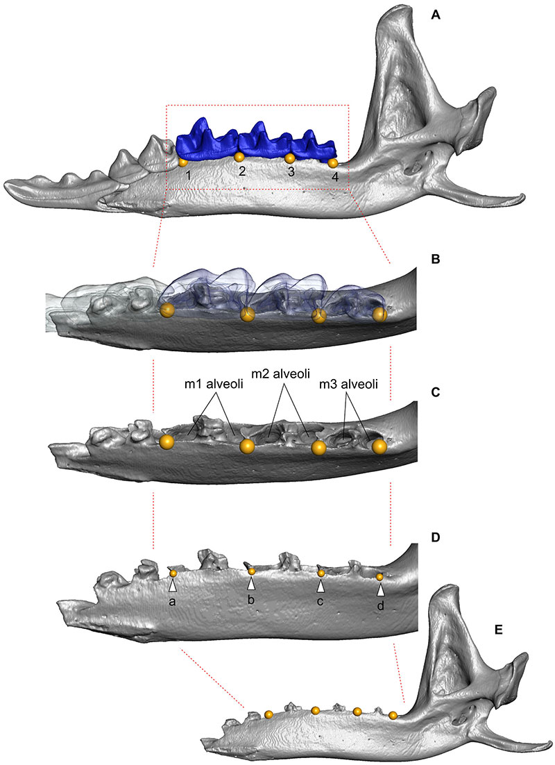
TABLE A3-1. Definition of landmarks used in the shape analysis of m1 (two-dimensional data).
| No. | Landmarks |
| 1 | Paraconid apex. |
| 2 | 'Paralophid bend' or a lowest point of the carnassial notch*. |
| 3 | Protoconid apex. |
| 4 | 'Protolophid bend' or a lowest point of the protocristid notch. |
| 5 | Metaconid apex. |
| 6 | Hypoconid apex. |
| 7 | Entoconid apex. |
* notches nomenclature by Lopatin (2006).
TABLE A3-2. Definition of landmarks used in the shape analysis of hemimandible (two-dimensional data). Abbreviation: lm (pl. lms), landmark; sm, semilandmark.
| No. | Landmarks |
| 1 | Anterior edge of the m1 anterior alveolus. |
| 2 | Anterior edge of the m2 anterior alveolus. |
| 3 | Anterior edge of the m3 anterior alveolus. |
| 4 | Medial point of the coronoid process apex. |
| 5 | Uppermost point of the condylar process. |
| 6 | Lowermost point of the condylar process. |
| sm 7-18 | Semilandmarks start at the posterior edge of the m3 posterior alveolus to frame-line of the uppermost position of the condylar process. The frame is strictly parallel to the base frame-line of the lower molar row. |
| sm 19-48 | Semilandmarks start at the frame-line of lm1 to the centrum of the notch of the lower dentary-angular process profile. The frame is strictly ortogonal to the base frame-line of the lower molar row. |
| Total: 48 lms. | |
FIGURE A3-2. m1 images preparation protocol. A, Two-dimensional images of m1 give from three-dimensional model of a hemimandible. B, Interface MorphoDig software (Lebrun, 2020) for work with the models. C, Model alignment to the 'Functional View' in sense to Polly (2003), see details in Figure A3-3. D, Obtaining separate images via 'Snipping Tool' for three repeats, A, B, and C. E, Landmarking ready images via tpsDig software (Rohlf, 2007). F, Obtaining three separate data sets required for assessing the 'metering error' influence or obtaining a final work data set as a mean between repeats. Abbreviations: a, b -- rotation along of the space planes for a model alignment.
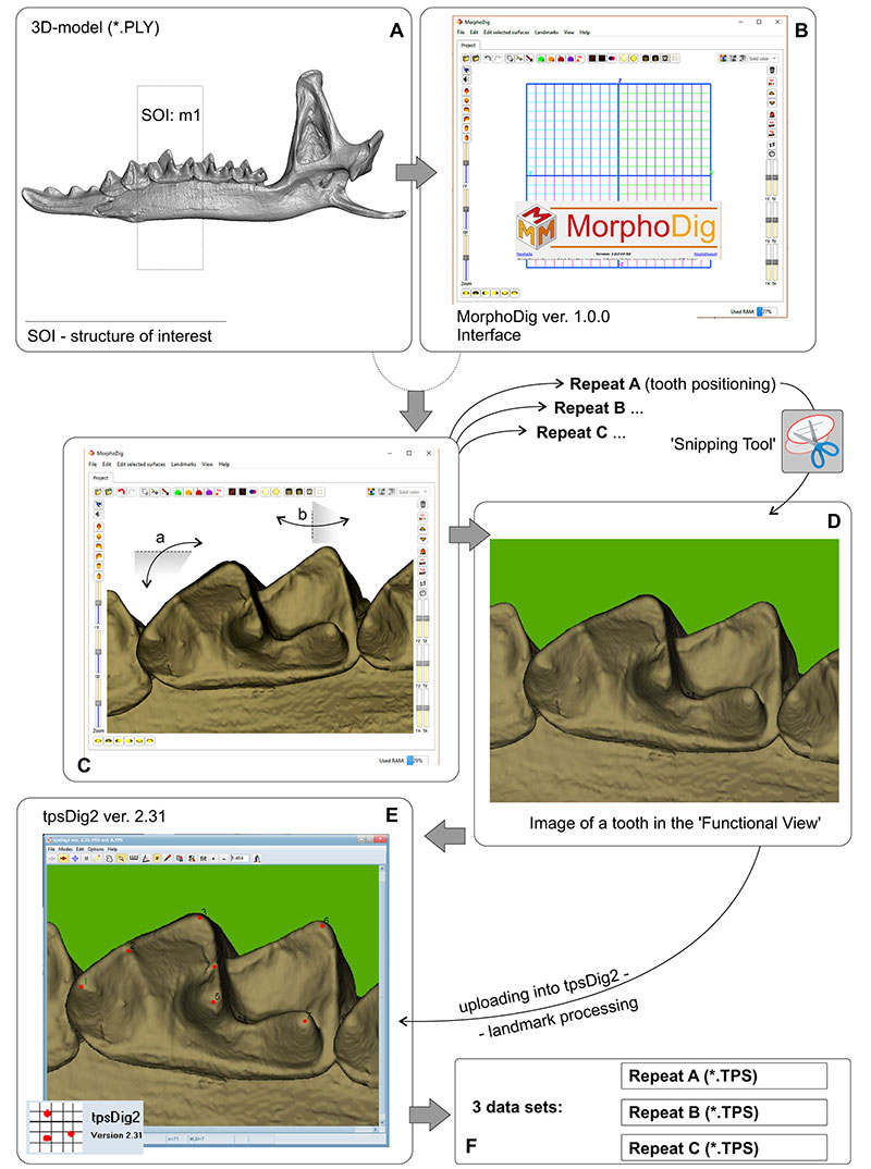
Note: A first study of the material from Serov and Pechora chromosomal races used geometric morphometry was implemented by Shchipanov et al. (2014). In the study m1 images obtained via digital camera combined with the binocular microscope. Against the 'metering error' influence, by the Polly (2003) recommendation, authors made five repeats of the separate images acquisition. In this study we tried to replace the image acquisition under microscope by the acquisition of images directly from 3D-models. The latter approach permits to reveal the key points of the correct/repeatable tooth alignment and controlling this through an application interface (e.g., MorphoDig). We admit this approach as an easier than alignment physical specimens under magnification, with one main limitation in three-dimensional models availability.
FIGURE A3-3. Key points of the m1 alignment into 'Functional View.' A, Reference image that prepared before a mass processing of the images (is opening during the image processing within a separate window for collation). B, Four key points that help m1 alignment: overall view of the paraconid and the anterior edge of m1; the functional view of the protoconid, i.e. the pre- and postprotocristid external edges hide a buccal surface of the trigonid; a view of the oblique cristid contact in manner of two planes as shown in C; and a shape (narrow triangle) of the posterobuccal surface of the talonid. D, m1 conids. Abbreviations: a, b -- planes of oblique cristid and the trigonid posterior border.
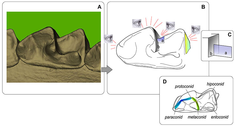
FIGURE A3-4. 'Specimen conglomerator' (SC). A, Autodesk 3Ds Max screen with three variants of conlomerator. B, The conglomerator dimensions supposed to be used 15 mL Falcon Centrifuge Tubes as a transportable container (Falcon used without cap). C, A view of four hemimandibles, scanned with SC in the CTVox software ver. 3.3.0 r1403 (64-bit) (Brucker microCT). D, Transversal digital section of SC, with the four mounted hemimandibles. E, An overall view of the Falcon tubes (source: https://www.amazon.in/Falcon-Centrifuge-Tubes-Polypropylene-352096/). Abbreviations: a -- SC with a cross-shaped bearing part (for 4, 8 or 12 small [width < 6 mm] items); b, c -- SC with a flatted bearing part (for 2 or 4 flat and width items, e.g., skull of tiny shrews); d -- a mounting area; e -- an inner diameter of SC that is inserted into the Falcon tube. An outer diameter (4 mm) serves as a cap; f -- a transversal section of the dentary; g -- a layer of the Dental Orthodontic Wax used for the bones mounting; h -- part of the cross-shaped SC. SC models in STL-format are available by the request (Leonid.Voyta@zin.ru).
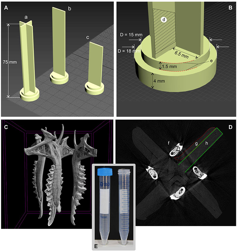
TABLE A3-3. Definition of landmarks used in the shape analysis of m1 (three-dimensional data).
| No. | Landmarks |
| 1 | Paraconid apex. |
| 2 | 'Paralophid bend' or a lowest point of the carnassial notch*. |
| 3 | Protoconid apex. |
| 4 | 'Protolophid bend' or a lowest point of the protocristid notch. |
| 5 | Metaconid apex. |
| 6 | Anterior end of the oblique cristid. |
| 7 | Oblique cristid bend. |
| 8 | Hypoconid apex. |
| 9 | Hypoconulid. |
| 10 | Entoconid apex. |
| sm 11-20 | Semilandmarks start at the posterobuccal angle of the crown base around to contact with sm 11 (by the basal torus 'more or less developed ridge'], see details in Voyta et al., 2022: figure 1). |
| Total: 50 lms. | |
REFERENCES
Lebrun, R. 2020. MorphoDig User's guide. Available at:
https://morphomuseum.com/tutorialsMorphoDig Accessed on 23 July 2023.
Lopatin, A.V. 2006. Early Paleogene insectivore mammals of Asia and establishment of the major group of Insectivora. Paleontological Journal, 40:205-405.
Polly, P.D. 2003. Paleogeography of Sorex araneus (Insectivora, Soricidae): molar shape as a morphological marker for fossil shrews. Mammalia, 68:233-243.
Rohlf, F.J. 2007. tpsDig2, version 2.31.
http://life.bio.sunysb.edu/morph/index.html Accessed on 23 July 2023.
Shchipanov, N.A., Voyta, L.L., Bobrtsov, A.V. and Kuprianova I.F. 2014. Intra-species structuring in the common shrew Sorex araneus (Lipotyphla: Soricidae) in European Russia: morphometric variability could give evidence of limitation of interpopulation migration. Russian Journal of Theriology, 13:119-140.
Voyta, L.L., Omelko, V.E., Tiunov, M.P., Petrova, E.A. and Kryuchkova, L.Yu. 2022. Temporal variation in soricid dentition: which are first - qualitative or quantitative features? Historical Biology, 34:901-1915.
https://doi.org/10.1080/08912963.2021.1986040
APPENDIX 4.
Statistic analysis results (additional information for metering error estimation).
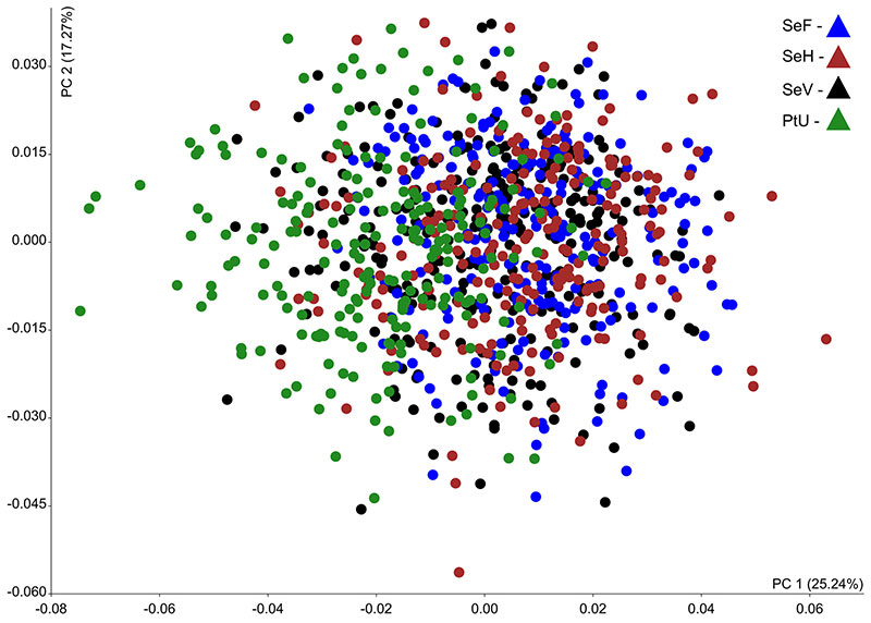
Variance Components Approach. Tables A4-1-A4-11 of appendix include result of the variance estimation of principal components of m1 data set (Variance Components Approach; Estimating method: ANOVA) under purpose of the metering error estimation. The estimation executed by two factors and them interaction: 'Sample' vs. 'Repeat.' Samples: SeV, SeF, SeH and PtU (see Tables 1 and 2, Figure 4 in the main text). Repeats: A, B and C. Total count of specimens is 759. Below provided 10 tabs, each included information for single PC. Calculated with Statistica 64 software ver. 10 (StatSoft). Red font marks statistically significance impact of the factors or interaction.
Table A4-1. Variance estimation of PC1.
| Effect | Univariate Tests of Significance for PC1 (Statistica_SP_dataset.sta) Over-parametrized model Type V decomposition |
|||||
| Effect (F/R) |
SS | Degr. of Freedom |
MS | F | p | |
| Intercept | Fixed | 0.021567 | 1 | 0.021567 | 84.7856 | 0.000000 |
| Repeat_Num | Fixed | 0.028113 | 1 | 0.028113 | 110.5213 | 0.000000 |
| Sample | Fixed | 0.074149 | 3 | 0.024716 | 97.1678 | 0.000000 |
| Error | 0.191794 | 754 | 0.000254 | |||
Table A4-2. Variance estimation of PC2.
| Effect | Univariate Tests of Significance for PC2 (Statistica_SP_dataset.sta) Over-parametrized model Type V decomposition |
|||||
| Effect (F/R) |
SS | Degr. of Freedom |
MS | F | p | |
| Intercept | Fixed | 0.001774 | 1 | 0.001774 | 8.39743 | 0.003866 |
| Repeat_Num | Fixed | 0.001795 | 1 | 0.001795 | 8.49862 | 0.003660 |
| Sample | Fixed | 0.011530 | 3 | 0.003843 | 18.19727 | 0.000000 |
| Error | 0.159248 | 754 | 0.000211 | |||
Table A4-3. Variance estimation of PC3.
| Effect | Univariate Tests of Significance for PC3 (Statistica_SP_dataset.sta) Over-parametrized model Type V decomposition |
|||||
| Effect (F/R) |
SS | Degr. of Freedom |
MS | F | p | |
| Intercept | Fixed | 0.001405 | 1 | 0.001405 | 7.25967 | 0.007509 |
| Repeat_Num | Fixed | 0.001506 | 1 | 0.001506 | 7.77926 | 0005418 |
| Sample | Fixed | 0.005956 | 3 | 0.001985 | 10.25855 | 0.000001 |
| Error | 0.145930 | 754 | 0.000194 | |||
Table A4-4. Variance estimation of PC4.
| Effect | Univariate Tests of Significance for PC4 (Statistica_SP_dataset.sta) Over-parametrized model Type V decomposition |
|||||
| Effect (F/R) |
SS | Degr. of Freedom |
MS | F | p | |
| Intercept | Fixed | 0.000104 | 1 | 0.000104 | 0.680992 | 0.409506 |
| Repeat_Num | Fixed | 0.000169 | 1 | 0.000169 | 1.107215 | 0.293025 |
| Sample | Fixed | 0.002843 | 3 | 0.000948 | 6.210660 | 0.000361 |
| Error | 0.115041 | 754 | 0.000153 | |||
Table A4-5. Variance estimation of PC5.
| Effect | Univariate Tests of Significance for PC5 (Statistica_SP_dataset.sta) Over-parametrized model Type V decomposition |
|||||
| Effect (F/R) |
SS | Degr. of Freedom |
MS | F | p | |
| Intercept | Fixed | 0.003776 | 1 | 0.003776 | 34.17823 | 0.000000 |
| Repeat_Num | Fixed | 0.004222 | 1 | 0.004222 | 38.21814 | 0.000000 |
| Sample | Fixed | 0.003093 | 3 | 0.001031 | 9.33138 | 0.000005 |
| Error | 0.083305 | 754 | 0.000110 | |||
Table A4-6. Variance estimation of PC6.
| Effect | Univariate Tests of Significance for PC6 (Statistica_SP_dataset.sta) Over-parametrized model Type V decomposition |
|||||
| Effect (F/R) |
SS | Degr. of Freedom |
MS | F | p | |
| Intercept | Fixed | 0.000005 | 1 | 0.000005 | 0.041768 | .838118 |
| Repeat_Num | Fixed | 0.000017 | 1 | 0.000017 | 0.145538 | 0.702944 |
| Sample | Fixed | 0.003352 | 3 | 0.001117 | 9.828267 | 0.000002 |
| Error | 0.085721 | 754 | 0.000114 | |||
Table A4-7. Variance estimation of PC7.
| Effect | Univariate Tests of Significance for PC7 (Statistica_SP_dataset.sta) Over-parametrized model Type V decomposition |
|||||
| Effect (F/R) |
SS | Degr. of Freedom |
MS | F | p | |
| Intercept | Fixed | 0.000003 | 1 | 0.000003 | 0.034734 | 0.852205 |
| Repeat_Num | Fixed | 0.000001 | 1 | 0.000001 | 0.005131 | 0.942917 |
| Sample | Fixed | 0.002731 | 3 | 0.000910 | 9.225604 | 0.000005 |
| Error | 0.074388 | 754 | 0.000099 | |||
Table A4-8. Variance estimation of PC8.
| Effect | Univariate Tests of Significance for PC8 (Statistica_SP_dataset.sta) Over-parametrized model Type V decomposition |
|||||
| Effect (F/R) |
SS | Degr. of Freedom |
MS | F | p | |
| Intercept | Fixed | 0.000082 | 1 | 0.000082 | 0.895817 | 0.344209 |
| Repeat_Num | Fixed | 0.000094 | 1 | 0.000094 | 1.021801 | 0.312416 |
| Sample | Fixed | 0.000939 | 3 | 0.000313 | 3.407021 | 0.017261 |
| Error | 0.069278 | 754 | 0.000092 | |||
Table A4-9. Variance estimation of PC9.
| Effect | Univariate Tests of Significance for PC9 (Statistica_SP_dataset.sta) Over-parametrized model Type V decomposition |
|||||
| Effect (F/R) |
SS | Degr. of Freedom |
MS | F | p | |
| Intercept | Fixed | 0.000293 | 1 | 0.000293 | 5.185180 | 0.023060 |
| Repeat_Num | Fixed | 0.000350 | 1 | 0.000350 | 6.183941 | 0.013107 |
| Sample | Fixed | 0.000049 | 3 | 0.000016 | 0.291419 | 0.831618 |
| Error | 0.042631 | 754 | 0.000057 | |||
Table A4-10. Variance estimation of PC10.
| Effect | Univariate Tests of Significance for PC10 (Statistica_SP_dataset.sta) Over-parametrized model Type V decomposition |
|||||
| Effect (F/R) |
SS | Degr. of Freedom |
MS | F | p | |
| Intercept | Fixed | 0.000111 | 1 | 0.000111 | 2.328022 | 0.127483 |
| Repeat_Num | Fixed | 0.000126 | 1 | 0.000126 | 2.639710 | 0.104641 |
| Sample | Fixed | 0.000016 | 3 | 0.000016 | 0.114755 | 0.951470 |
| Error | 0.036079 | 754 | 0.000048 | |||
FIGURE A4-1. Result of principal component analyses based on the m1 shape. The tooth data represented as three repetition of four samples within space of PC1 and PC2: SeV, SeF, SeH and PtU.
An Example of Underestimated Metering Error. Image based on the data published by Zazhigin and Voyta (2019: supplemental materials).
FIGURE A4-2. Measurements of the m1 and m2 of Beremendiini specimens: A. Common graph for eight species (by Zazhigin and Voyta, 2019, with changes); B Magnified part of graph with variability area of European samples of B. fissidens (dark grey convex hull as for A, original material of B. fissidens (three- and four-digit numbers), Lunanosorex lii (Ll), B. pohaiensis (Pph), B. pliocaenica (Ppl); C. Measurements for each holotype. Abbreviations: Bf_B5 -- B. fissidens from Beremend 5 locality (Hungary; late Pleistocene); L(m1) -- m1 length; L(m2) -- m2 length; Ll_QP -- L. lii from Qipanshan Hill locality (China; late Pliocene); Ll_HX -- L. lii from Houxushan Hill locality (China; late Pliocene); Pph_h1 -- holotype dimensions from original description of B. pohaiensis; Pph_h2 -- holotype of B. pohaiensis re-dimensions by Jin and Kawamura (1996); Pph_HAI -- B. pohaiensis from Haimao locality (China; early Pleistocene); Pph_r -- re-demensions of replicated B. pohaiensis holotype by Zazhigin and Voyta (2019); Ppl_h4 -- holotype dimensions from original description of B. pliocaenica; Ppl_h5 -- re-dimensions of B. pliocaenica holotype by Jin, Kawamura (1996).
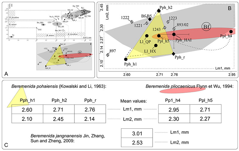
TABLE A4-11. Comparison of m1 measurements by 2D-images and 3D-models. Measurements are mean values with limits. * -- see Figure 1 and Appendix 1.
| Locality | lingual Lm1 (2D-images) |
lingual Lm1 (3D-models) |
| S. araneus | ||
| SeF (n = 15) | 1.49 (1.43-1.54) | 1.49 (1.45-1.53) |
| SeH (n = 15) | 1.54 (1.50-1.63) | 1.51 (1.48-1.65) |
| SeV (n = 15) | 1.51 (1.47-1.57) | 1.48 (1.46-1.52) |
| PtU (n = 55) | 1.53 (1.37-1.54) | 1.47 (1.36-1.55) |
| Dan' subsample S. araneus (n = 6) | 1.44 (1.38-1.48) | 1.42 (1.39-1.44) |
| Sim3 subsample S. araneus (n = 6) | 1.55 (1.50-1.60) | 1.51 (1.36-1.62) |
| Cher 1 (n = 5) | 1.52 (1.48-1.56) | 1.52 (1.45-1.60) |
| DKS3 subsample S. araneus (n = 5) | 1.55 (1.50-1.59) | 1.54 (1.50-1.61) |
| S. tundrensis | ||
| Dan' subsample S. tundrensis (n = 6) | 1.42 (1.35-1.48) | 1.40 (1.37-1.45) |
| S. tundrensis(T1-T7)* (n = 20) | 1.41 (1.29-1.49) | 1.39 (1.30-1.49) |
| Sim3 subsample S. tundrensis (n = 2) | 1.47 (1.43, 1.52) | 1.51 (1.45, 1.57) |
| DKS3 subsample S. tundrensis (n = 8) | 1.37 (1.34-1.42) | 1.37 (1.33-1.40) |
APPENDIX 5.
Shape analysis supporting information.
Skull Shape. For the purpose of undoubted species identification, we applied a skull shape analysis follow Klingenberg (2011). We applied the same images preparation (ventral view of the skull obtained via Epson Perfection flatbed scanner with 2400 dpi resolution) and same landmarks set (22 true landmarks for the left side of the skull). The shape analyses executed with MorphoJ Application ver. 1.06d Shchipanov et al. (2014). Analysis performed for two target samples: PtU and Dan,' together with two reference samples of S. araneus (SeV) and original geographical samples of S. tundrensis (Appendix 1).
Landmarks Definition:
1. Most posterior point of the foramen magnum aperture.
2. Most anteriro point of the foramen magnum aperture.
3. Point of the caudal opening of the pterygoid canal.
4. Most posterior point of the palatinum (on the postpalatine torus).
5. Most anteriro point of the palatinum;
6. Most posterior point of the premaxilla in the ventral view.
7-11. Tips of the upper antemolars (A1-A5).
12. Buccal border between A5 and P4.
13. Tip of protocone of M1.
14. Buccal border between P4 and M1.
15. Tip of protocone of M2.
16. Buccal border between M1 and M2.
17. Tip of protocone of M3.
18. Buccal border between M2 and M3.
19. Foramen ovale (the formal border of the rostral part and braincase).
20. Most lateral point of the braincase outline.
21. Most postero-lateral poin of the basioccipital-petrosum connection.
22. Tip of the paracondylar process.
Result (see Figure A5-1 below and the main text). Whole sample PtU, except single specimen (ZIN 107849/1063), has been associated with S. araneus. Dan' sample partly divided to S. tundrensis (ZIN 107852/727, /957, /1089, /1129, /1182, /1221; n = 6), partly to S. araneus (ZIN 107851/711, /954, /1133, /1536, /1562; n = 5; single specimen from Ramen'e ZIN 107850/1189 calculated within Dan' sample).
REFERENCES
Shchipanov, N.A., Voyta, L.L., Bobretsov, A.V. and Kuprianova, I.F. 2014. Intra-species structuring in the common shrew Sorex araneus (Lypotyphla: Soricidae) in the European Russia: morphometric variability could give evidence of limitation of interpopulation migration. Russian Journal of Theriology, 13:119-140.
Klingenberg, C.P. 2011. MorphoJ: an integrated software package for geometric morphometrics. Molecular Ecology Resources, 11:353-357.
FIGURE A5-1. Results of the principal component analysis based on the skull shape, combined of S. araneus and S. tundrensis samples. A. Morphospace within PC1-2 with clear separation both species; B1. Skull shape (in ventral view) in a transformation frame on the negative end of PC1 that corresponding to S. tundrensis; B2. Skull shape (in a transformation frame on the positive end of PC1 that corresponding to S. araneus. Abbreviations: A1-A5 -- upper antemolar row; Dan' -- Dan' sample; for. ovale -- foramen ovale (lm19); I1 -- first upper incisor; lm -- landmark; M -- upper molar; P4 -- fourth upper premolar; pal -- palatinum; PtU -- Ulashevo sample (Pechora race); SeV -- reference sample of S. araneus; tdr -- reference sample of S. tundrensis; zpmx -- zygomatic process of the maxilla.
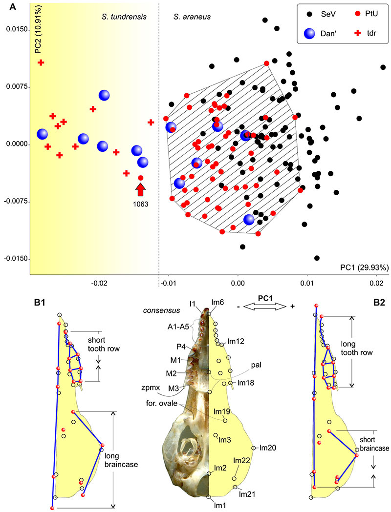
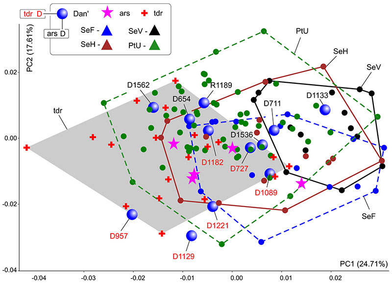
FIGURE A5-2. Results of the principal component analysis based on the hemimandible shape dataset, combined of S. araneus and S. tundrensis samples. Samples dispersion displayed as convex hulls. Key: ars, specimens of S. araneus from 'non-chromosomal' samples; Dan'(D), sample of S. tundrensis from Dan' village; tdr, S. tundrensis. See the main text and Figure 5B.
APPENDIX 6.
PHYLOMORPHOSPACE ANALYSIS AND SCHLAGER'S VISUALIZATION
Phylogenetic Analysis
Sampling and GenBank Information. For the calculation of the phylogenetic signal we used 12 soricine species: Sorex cinereus (ZIN 71061), S. alpinus (ZIN 34077), S. araneus (ZIN 70532), S. asper (ZIN 65185), S. tundrensis (ZIN 90408), S. daphaenodon (ZIN 11428), S. volnuchini (ZIN 26266), S. buchariensis (37206), S. minutus (ZIN 84257), S. gracillimus (5360), S. minutissimus (ZIN 98582) (ingroup) and Neomys fodiens (outgroup). All 3D-models of isolated m1 and m2 available in the MorphoBank Project P4500 "A morphospace dynamics from past to present through the modern geometric morphometric approaches" at: http://www.morphobank.org
For the particular analyses represented on Figure 10 (see the main text) used 7 species: Sorex cinereus, S. alpinus, S. araneus, S. tundrensis, S. minutus, S. minutissimus (ingroup) and Neomys fodiens (outgroup).
We used the following seven genes accessed in GenBank:
cytB: AB175120, AY014952, HM036155, MH332354, GU564816, MH332368, MH332333, MH332353, MH332358, MH332342, HM992669, GU981295.
ApoB: MH332007, MH331999, MH332030, MH332024, MH332037, MH332041, MH332043, MH332050, MH332054, HM992797, MH331994, GU981130.
BRCA1: MH332085, MH332078, HM036123, MH332099, MH332094, MH332105, MH332108, MH332110, MH332118, MH332122, HM992720, KP995400, MH332074, GU981205.
BRCA2: MH332146, MH332175, MH332169, MH332164, MH332182, MH332185, MH332187, MH332194, MH332198.
RAG2: MH331924, MH331918, MH331949, MH331944, MH331937, MH331956, MH331960, MH331961, MH331968, MH331972, MH331913, GU981463.
IRBP: MH332280, MH332274, MH332298, MH332294, MH332287, MH332305, MH332308, MH332310, MH332314, MH332317.
GHR: MH332222, MH332219, MH332243, MH332237, MH332233, MH332247, MH332250, MH332252, MH332256.
FIGURE A6-1. Consensus tree based on the seven concatenated genes data set.
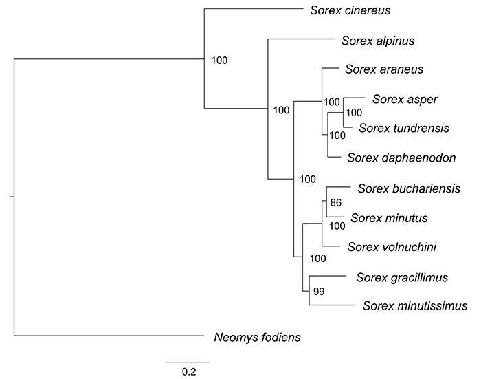
Phylogeny and Shape Analysis (Phylogenetic Signal Assessment). As a basis for phylogenetic analyses we used the phylogeny of Sorex species of Bannikova et al. (2018). For the phylogenetic analyses used Bayesian Inference. Gene sequences of 12 species were aligned in Geneious Prime 2019.1 using Geneious alignment with default settings. The phylogenetic reconstruction of Sorex genus was performed in MrBayes 3.2.6 (Ronquist et al., 2012). The full tree represented below. For the particular analyses represented on Figure A6-1 we used reduced tree for 7 species.
To quantify the phylogenetic signal through a multivariate method that developed by Adams (2014) we used 'Geomorph' (Adams et al., 2023]) and 'Ape' (Paradis and Schliep, 2019) packages of the R environment.
R-packages. The phylogenetic signal has been computed with a function 'physignal' from Geomorph Package (Adams et al., 2023); also used Ape Package (Paradis and Schliep, 2019).
Visualization
3D-models. Sorex tundrensis (ZIN 90408) was determined as a reference object for visualization procedure. This specimen was also determined as a Target 1; S. araneus (ZIN 70532) was determined as a Target 2.
The procedure description and all details, including the R-script, were provided in the published study by Voyta et al. (2022).
Landmarking. The landmarks were prepared using MorphoDig ver. 1.6.0 software (Lebrun, 2020).
REFERENCES
Adams, D.C. 2014. Generalized K statistic for estimating phylogenetic signal from shape and other high-dimensional multivariate data. Systematic Biology, 63:685-697.
Adams, D.C., Collyer, M., Kaliontzopoulou, A. and Baken, E. 2023. Package ‘geomorph’, Version 4.0.5. Available at:
https://cran.r-project.org/web/packages/geomorph/geomorph.pdf
Adler, D. and Murdoch, D. 2021. Package ‘rgl’, Version 0.104.16. Available at:
https://cran.r-project.org/web/packages/rgl/rgl.pdf
Bannikova, A.A., Chernetskaya, D., Raspopova A., Alexandrov, D., Fang, Y., Dokuchaev, N., Sheftel, B. and Lebedev, V. 2018. Evolutionary history of the genus Sorex (Soricidae, Eulipotyphla) as inferred from multigene data. Zoologica Scripta, 47:518-538.
Hulme-Beaman, A., Claude, J., Chaval, Y., Evin, A., Morand, S., Vigne, J.D., Dobney, K. and Cucchi, T. 2019. Dental shape variation and phylogenetic signal in the Rattini tribe species of mainland Southeast Asia. Journal of Mammalian Evolution, 26:435-446.
Lebrun, R. 2020. MorphoDig User's guide. Available at:
https://morphomuseum.com/tutorialsMorphoDig Accessed on 23 July 2023.
Paradis, E. and Schliep, K. 2019. Ape 5.0: An environment for modern phylogenetics and evolutionary analyses in R. Bioinformatics, 35:526-528.
https://doi.org/10.1093/bioinformatics/bty633
Ronquist, F., Teslenko, M., van der Mark, P., Ayres, D.L., Darling, A., Höhna, S., Larget, B., Liu, L., Suchard, M.A. and Huelsenbeck, J.P. 2012. MrBayes 3.2: efficient Bayesian phylogenetic inference and model choice across a large model space. Systematic Biology, 61:539-542.
Schlager, S. 2017. Morpho and Rvcg - Shape Analysis in R: R-packages for geometric morphometrics, shape analysis and surface manipulations, p. 217-256. In Zheng, G., Li, S. and Szekely, G. (eds.), Statistical Shape and Deformation Analysis, 1st. Edition. Academic Press Inc., San Diego.
Terray, L., Denys, C., Goodman, S.M., Soarimalala, V., Lalis, A. and Cornette, R. 2022. Skull morphological evolution in Malagasy endemic Nesomyinae rodents. PLoS ONE, 17:e026304.
Voet, I., Denys, C., Colyn, M., Lalis, A., Konečny, A., Dlapré, A., Nicolas, V. and Cornette, R. 2022. Incongruences between morphology and molecular phylogeny provide an insight into the diversifcation of the Crocidura poensis species complex. Scientific Reports, 12:e10531.
Voyta, L.L., Abramov, A.V., Lavrenchenko, L.A., Nicolas, V., Petrova, E.A. and Kryuchkova, L.Y. 2022. Dental polymorphisms in Crocidura (Soricomorpha: Soricidae) and evolutionary diversification of crocidurine shrew dentition. Zoological Journal of the Linnean Society, 196:1069-1093.
