FIGURE 1. A: Schematic drawing of a CCD-type flatbed scanner. B-C: Schematic drawing of a glossy metal sphere scanned with a flatbed scanner, used to approximate the angle in which the light of the lamp of the carriage unit illuminates the subject. B: Sphere as scanned, corresponds to a bottom-up view in A. C: Sphere inside view (enlarged and version of its depiction in A ), upper portion cropped. Abbreviations: a, distance of the centre of the specular highlight (along the scanning direction) towards the centre of the sphere (both measured in a flat projection); r, radius of the sphere; θ, angle between the light coming from the lamp and the light reflected from the metal sphere perpendicular to the scanner surface.
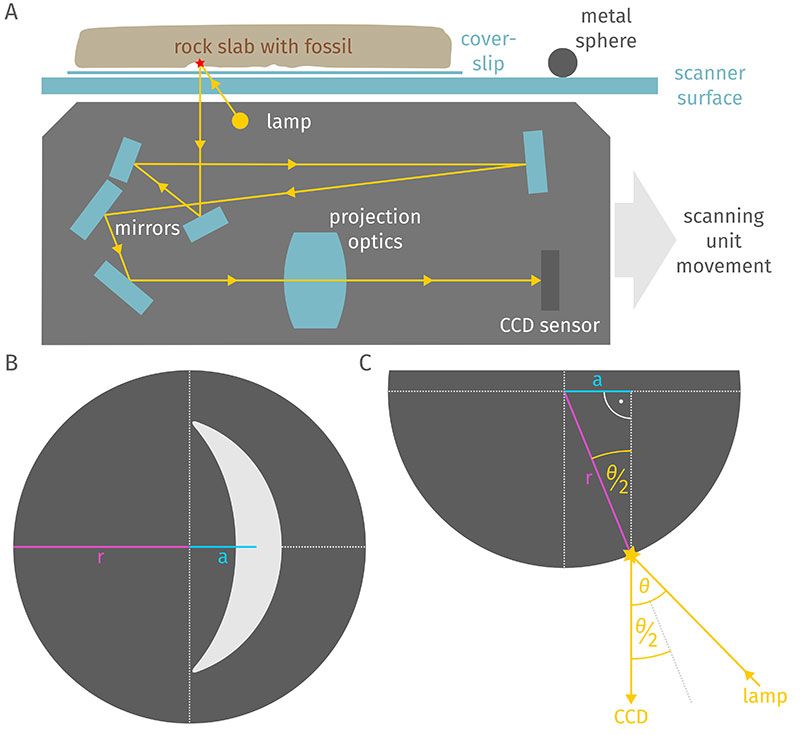
FIGURE 2. Schematic drawings of different methods to achieve stereoscopic imagery (stereo image pairs, stereo anaglyphs, or wiggle images), not to scale. Note the similarity between the approaches in B, D, and E. A: Tilting of a camera relative to a subject, may require recording a focus stack to compensate for misalignment of fossil surface and focal plane (red dotted lines). B: Translation of a subject within the view of a camera (b, “stereo base”), resulting in a change of the viewing angle (γ) for a given distance (d) between the optical centre of the lens and the subject. C: Viewing angles in CCD type scanners, relationship between distance (b) to the midline of the scanner and the viewing angle onto the subject (γ) for different lengths (d). Note that the further away a subject is from the midline, the more translation is required to affect the viewing angle. D: Translation of a camera relative to a subject. E: Translation of a subject on a CCD-type flatbed scanner, perpendicular to the carriage movement. F: Schematic depiction of a flatbed scanner window (blue), on which a subject (grey) is moved perpendicular to the movement of the sensor and the lighting (yellow).
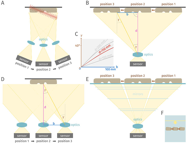
FIGURE 3. Schematic representation of the alignment process used for creating Multi Light Image Collections using a flatbed scanner. The direction of the light relative to the imaged subject is depicted by a yellow arrow and a dark grey sphere with a specular highlight. Enlarged dark grey spheres represent superimposed views of the spheres in all images before and after the alignment. A: Images as recorded. B: Images after alignment.
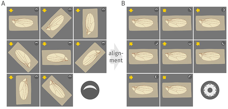
FIGURE 4. Comparison between stereo pairs and anaglyphs created using images from a flatbed scanner and depth profiles retrieved from a digital microscope. Fossil beetle from the Miocene of Öhningen, GPIT-PV-40359. A: Micrograph created with a digital microscope, pink and blue lines depicting to-scale height profiles along the corresponding dotted lines. B-C: Images retrieved from a flatbed scanner, left and right image differ by a displacement of 50 mm perpendicular to the carriage unit movement. Bl -Br: Stereo pair suitable for parallel viewing. C: Red-cyan stereo anaglyph suitable for viewing with stereo glasses. D: Height map created by a digital microscope (depth from de-focus), bright areas are higher than dark areas. E-F: Images retrieved from a flatbed scanner, left and right image differ by a displacement of 160 mm perpendicular to the carriage unit movement. Bl -Br: Stereo pair, suitable for parallel viewing. C: Red-cyan stereo anaglyph, suitable for viewing with stereo glasses.
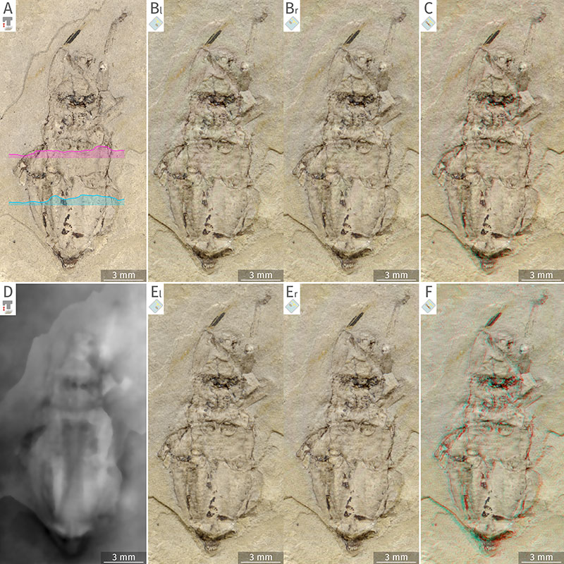
FIGURE 5. Comparison between stereo pairs and anaglyphs created by tilting the optical apparatus of a digital microscope and anaglyphs created using images retrieved from a flatbed scanner. Fossil beetle from the Miocene of Öhningen, GPIT-PV-40359. A-B: Images created by tilting the optical apparatus 10 degrees to the left and 10 degrees to the right (20 degrees between the views). Al -Ar: Stereo pair suitable for parallel viewing. B: Red-cyan stereo anaglyph, suitable for viewing with stereo glasses. C: Red-cyan stereo anaglyph based on a stereo pair recorded using a flatbed scanner, translation of 50 mm perpendicular to the scanning movement. D-E: Images created by tilting the optical apparatus 20 degrees to the left and 20 degrees to the right (40 degrees between the views). Dl -Dr: Stereo pair suitable for parallel viewing. E: Red-cyan stereo anaglyph. F: Red-cyan stereo anaglyph based on a stereo pair recorded using a flatbed scanner, translation of 160 mm perpendicular to the scanning movement.
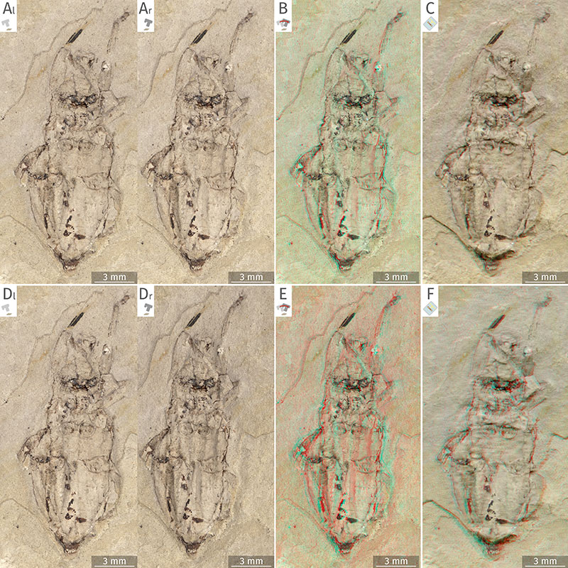
FIGURE 6. Different fossil insect remains, images retrieved using a flatbed scanner and normal maps produced using rotated flatbed scanner images, yellow arrows depicting the directions of illumination, circular colour legends depicting how spheres would appear in the normal maps. A-B: Fossil beetle from the Miocene of Öhningen, GPIT-PV-112875. A: Flatbed scanner image. B: Normal map based on 16 images. C-D: Fossil larva of a dragonfly from the Miocene of Öhningen, GPIT-PV-112869. C: Flatbed scanner image. D: Normal map based on 16 images. E-F: Fossil forewing of a grasshopper from the Miocene of Öhningen, GPIT-PV-112874. E: Flatbed scanner image. F: Normal map based on 4 images. G-H: Fossil wing of a dragonfly from Braunschweig, GPIT-PV-112870. G: Flatbed scanner image. H: Normal map based on four images.
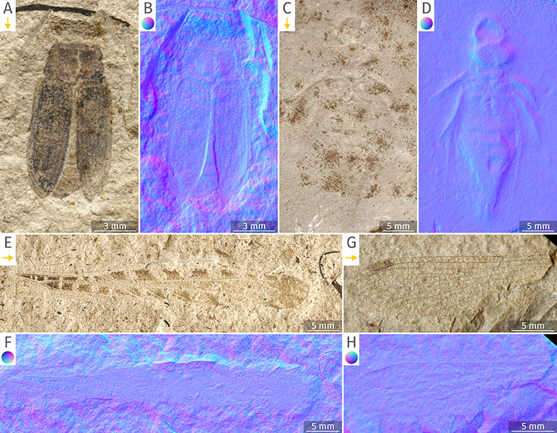
FIGURE 7. Fossil insect from the Miocene of Öhningen GPIT-PV-112875, white arrows denote areas with distinctly visible quality differences between the normal maps. A: Image retrieved using a flatbed scanner, yellow arrow depicts the illumination direction, pink line depicts a to-scale height profile along the corresponding straight dotted line. B-F: Normal maps created using images retrieved from a flatbed scanner by rotating the specimen in equal steps, circular colour legend depicts how a sphere would appear in the normal map. B: Normal map from three images. C: Normal map from 4 images. D: Normal map from eight images. E: Normal map from 16 images. F: Detail of the head, normal map from 16 images (cropped and enlarged version of E. G: Detail of the head (same field of view as F), normal map retrieved from a ring light setup with eight LEDs, focus-merged normal maps from 27 focus levels.
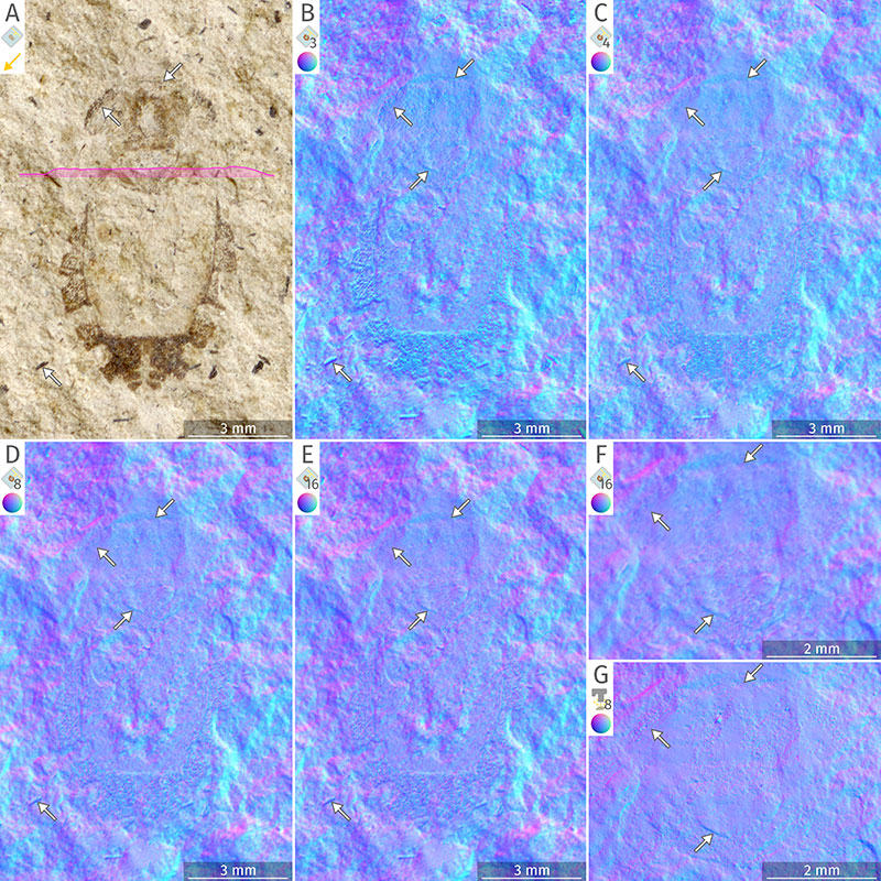
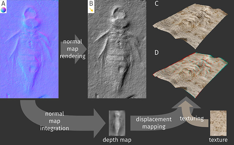
FIGURE 8. Examples of visualisations that can be derived from normal maps, including a schematic overview of the workflow to obtain the graphics. Fossil larva of a dragonfly from the Miocene of Öhningen, GPIT-PV-112869 (see also Figure 6 C-D). A: Normal map reconstructed from 16 images. B: Artificial light scene rendering, light from upper left side at a 20-degree angle to the image, artificially reduced surface roughness, normal map as the only image information source, orthographic view. C: Visualisation of the depth map (generated from the normal map, bottom centre), with original image colour information (one of the scanned images, bottom right), rendered 3D scene, perspective view. D: Same as C but rendered as a stereoscopic image, red-cyan stereo anaglyph.