Artificial bivalves

Artificially evolved functional shell morphology of burrowing bivalves

Daniel P. Germann, Wolfgang Schatz, and Peter Eggenberger Hotz

Article number: 17.1.8A
https://doi.org/10.26879/394
Copyright Palaeontological Association, February 2014

Author biographies
Plain-language and multi-lingual abstracts
PDF version

Submission: 11 April 2013. Acceptance: 19 December 2013

{flike id=649}

ABSTRACT

The morphological evolution of bivalves is documented by a rich fossil record. It is believed that the shell shape and surface sculpture play an important role for the burrowing performance of endobenthic species. While detailed morphometric studies of bivalve shells have been done, there are almost no studies experimentally testing their dynamic properties. To investigate the functional morphology of the bivalve shell, we employed a synthetic methodology and built an experimental setup to simulate the burrowing process. Using an evolutionary algorithm and a printer that prints three dimensional (3D) objects, the first ever artificial evolution of a physical bivalve shell was performed. The result was a vertically flattened shell occupying only the top sediment layers. Insufficient control of the sediment was the major limitation of the setup and restricted the significance of the results. Nevertheless, it is demonstrated that systematic palaeontological research may substantially profit from synthetic methods. We suggest investigating functional morphologies not only by emulating the dynamical processes but also evolutionary pressure using evolutionary algorithms.

Daniel P. Germann. Artificial Intelligence Laboratory, Department of Informatics, University of Zürich, Andreasstrasse 15, 8050 Zürich, Switzerland, germann@ifi.uzh.ch
Wolfgang Schatz. Academic Services Centre, University of Lucerne, Pfistergasse 20, 6003 Luzern, Switzerland, Wolfgang.Schatz@unilu.ch
Peter Eggenberger Hotz. Mærsk-McKinney-Møller Institute, University of Southern Denmark, Campusvej 55, 5230 Odense M, Denmark, petereggenbergerhotz@gmail.com

Keywords: burrowing bivalves; functional morphology; artificial evolution; evolutionary pressure; biomechanics; morphospaces

Final citation: Germann, Daniel P., Schatz, Wolfgang, and Eggenberger Hotz, Peter. 2014. Artificially evolved functional shell morphology of burrowing bivalves. Palaeontologia Electronica Vol. 17, Issue 1;8A; 25p. https://doi.org/10.26879/394
palaeo-electronica.org/content/2014/649-artificial-bivalves

INTRODUCTION

Bivalves constitute about a ninth of the known fossil record (Amler et al., 2000). Periods of fast radiation and drastic morphological changes, e.g., due to the appearance of siphons in the post-Palaeozoic or to the transition from hard to soft substrates, alternated with periods of only minor modifications to the shell (Seilacher, 1984; Stanley, 1968). It has been repeatedly shown that the shell morphology is adapted to effective locomotion through the sediment (Stanley, 1975a), e.g., by becoming more streamlined and elongated (Seilacher, 1984; Watters, 1993), by reducing back-slippage and forward friction using terrace-shaped commarginal ridges (Savazzi and Huazhang, 1994; Seilacher, 1984), by using discordant ridges (Stanley, 1969) or by adjusting the sculpture to the sediment grain size (de la Huz et al., 2002; Savazzi and Huazhang, 1994).

To burrow themselves into the sediment, bivalves use a two-anchor system. The shell and the foot – a muscular part of the soft body ventrally protruding out of the shell – alternately anchor the bivalve in the sediment, while the other one is moved forward. Anchoring is done by increasing the size: the shell is opened and presses against the sediment, the foot swells through an increase in blood pressure. By the anterior and posterior retractor muscles the shell is pulled closer to the anchored foot. The sequential contraction of these muscles leads to a characteristic rocking motion of the shell. The rotation around two separate rotation axes leads to a net downward motion. When the valves are contracted to release anchoring and to inflate the foot, water is expelled from the mantle cavity between the valves loosening the sediment and thus decreasing the resistance to penetration. The whole process is called "burrowing sequence" and was first described by Trueman (1966).

The (functional) morphology of bivalves may be analysed using different approaches (e.g., Crampton, 1995). Often, morphometric analyses are based on landmarks, i.e., salient points of the shell morphology such as the beak, valve adductor muscle scars etc. (Adams et al., 2004; Bookstein, 1997; Dryden and Mardia, 1998).

Another approach uses virtual growth processes to generate shell geometries. They use the fact that bivalve shells – as the shells of gastropods – have a convoluted shape following a logarithmic spiral due to an accretionary growth process. One of the first attempts to mathematically model this process was done by Raup and Michelson (1965), where also the term "theoretical morphology" was introduced. Since then, many different approaches have been suggested, most of which are based on a simple growth process that produces a sequence of closed profile curves of increasing size that travel along a three-dimensional helicospiral (Fowler et al., 1992; Hammer and Bucher, 2005; Okamoto, 1988). With these approaches, only few parameters are needed to generate realistic virtual shell shapes.

To systematically analyse and compare different shell morphologies, a theoretical morphospace can be constructed from the morphological parameters. The theoretical morphospace is a multidimensional space where the dimensions correspond to the parameters and each individual shape is represented as a point (McGhee, 1999). While the theoretical morphospace spans the whole space of possible morphologies using a given set of parameters, the actual morphospace is the set of points representing specimens actually found in nature (McGhee, 1999).

While morphometric measures can be extracted from fossils, it is not possible to adequately assess the function of the morphological traits since no living specimens can be observed. Conclusions may be drawn by analogy from similar recent species, but these studies are restricted to the available specimens and may not properly reflect the details of the fossil morphology. To adequately assess the function of the morphological traits, it would be necessary to watch the fossil species in action.

In this paper we present an experimental platform to test different bivalve shell morphologies in terms of their burrowing performance. A synthetic methodology is followed by generating arbitrary artificial shell shapes and materializing them using a 3D printer. They are then tested in an artificial burrowing environment to better understand the function of the morphological traits. We also report the results of the first ever experiment to evolve physical shell morphologies based on burrowing performance. We propose artificial evolutionary systems as a tool to study evolutionary pressure on functional morphology.

The synthetic approach has been increasingly productive in fields such as biomimetics, biorobotics and artificial life (Langton, 1989; Webb, 2000). Also the emulation of evolution has proved both insightful and useful in many areas (Bäck, 1997; Fogel, 1998). Evolutionary algorithms have been used to optimize technical systems (Bentley, 1999; Rechenberg, 1973, 2000) or to evolve controllers of robots (Floreano et al., 2008). Also morphologies of artificial organisms have been evolved in software (Eggenberger Hotz, 2003; Sims, 1994) or, as manufacturing processes become faster and cheaper, hardware (Lipson and Pollack, 2000).

Two examples of the synthetic approach applied to study bivalve burrowing are described by Stanley (1975b) and Winter et al. (2012). Stanley used a cast of Mercenaria mercenaria to demonstrate the effect of the blunt anterior area of its shell. By decreasing back-slippage, it moved the rotation axes of the rocking motion outwards and thus increased the downward motion of the shell. Winter built a technical drilling device inspired by the bivalve Ensis directus and demonstrated its reduced energy consumption compared to traditional devices. He also investigated the localized fluidization of the sediment around the shell due to valve contraction.

Most biomimetic research has two aspects: a) to draw inspiration from nature to build better technical artefacts; and b) to use a synthetic approach to better understand natural phenomena and organisms. Often the focus lies on the first aspect, especially in the case of artificial evolution that is used as a bio-inspired optimization tool. In this paper we focus on the second aspect and suggest expanding the synthetic methodology by using evolutionary algorithms to study the evolutionary pressure on the functional morphology of burrowing bivalves.

In this paper, we describe the experimental setup including the morphological shell model and the evolutionary algorithm. We also present the results of a morphological evolution experiment performed with the setup.

MATERIALS AND METHODS

The setup consisted of an environment of underwater sandy sediment, models of bivalve shells and an external actuation system that induced a rocking burrowing motion on the shells. During the evolutionary experiment, the morphology of the shells changed according to a fitness function based on the burrowing performance. A more detailed description of the setup used in this study was published in Germann and Carbajal (2013). Compared to an earlier version of the setup (Koller-Hodac et al., 2010), it featured technical improvements like a modular approach to switch bivalve shell models or an improved control program that used force control instead of position control (Germann and Carbajal, 2013) to make the burrowing process more realistic.

Setup

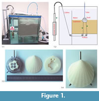Bivalve burrowing was mimicked using the experimental setup shown in Figure 1. The cubic water tank (side length 60 cm) contained a compartment with well-rounded quartz sand (grain size 0.7–1.2 mm, bulk density 1500 kg/m³).

Bivalve shells were assembled from two 3D-printed ABS (acrylonitrile butadiene styrene) plastic valves and a central metal disc. Depending on the type of feature, the resolution of the printer was between 0.1 and 0.5 mm. We found that the abrasion of the ABS-shells by the sand was negligible (<0.5 mm at the shell front after more than 280 burrowing runs).

Using a 3D printer allowed the materialization of any shell morphology generated by the evolutionary algorithm. To create one valve of a shell, an outer shell surface was combined with an inner attachment structure featuring a bayonet coupling mechanism (Figure 1.3). This mechanism allowed the attachment to a central metal disc. The disc had two attachment sites for the actuation mechanism at the bottom and a water supply duct at the top (Figure 1.2-4). Water pumped into the shell and ejected through holes along the ventral edge could be used to imitate water expulsion. However, in this study, the water expulsion system was not used. The water supply tube was still attached to all shells to maintain comparability to other experiments and to ensure an erect standard orientation of the shells at the beginning of the experiments.

The shells were attached to the outside actuation system by two coated steel cables (diameter 1.2 mm) that simulated the force of the foot retractor muscles of natural bivalves. One cable was attached to the anterior part of the shell, one to the posterior part. The setup did not feature any further representation of the foot. Experiments were performed by pulling the artificial shells into the sediment using a rocking motion induced by alternate pulling of the cables. These were deviated through the sediment via pulleys and attached to two linear motors mounted vertically at the outside of the tank (Figure 1.2).

The burrowing process was simulated by an open-loop control program on the controllers of the linear motors. Each motor executed a sequence of single burrowing steps. By adding a short time lag for the second motor a rocking motion of the shell was induced, which rotated the shell first in anterior and then in posterior direction. A burrowing step consisted of a pulling and a waiting phase. During the pulling phase, a fixed pulling force was applied to the cable. During the waiting phase, the position of the motor sliders and therefore of the shell was held constant by PID (proportional-integral-derivative) control. A maximal step size was maintained by switching to the waiting phase early as soon as a predetermined limit was reached. The total step duration was held constant by adapting the waiting phase duration.

For the experiments of this study, we used the following configuration: applied pulling force: 130 N (with measured peaks up to 200 N), pulling phase duration: 400 ms, maximal step size: 12 mm, waiting phase duration: 1 s, number of steps: 15, time lag of the second motor: 200 ms. Burrowing depth as a function of burrowing time saturated, i.e., the actually performed steps became smaller with increasing depth until the shell did not move any more (Germann and Carbajal, 2013).

The internal slider position signals of the motors and signals from force sensors inserted between the slider ends and the cables were recorded for all experiments. The slider positions were systematically overestimating the burrowing depth by (6.4 ± 2.2)% (mean ± standard deviation, n = 400) due to deformations of the setup under cable tension, but did not change the relative performance of the different shells. Throughout this paper we use "burrowing depth" to mean "slider position."

Parameters determining the configuration of the setup for each experiment can be divided into a) environmental parameters (such as grain size); b) motion parameters (as mentioned above); and c) morphological parameters. Experiments reported here did only vary the morphological parameters of the shell.

Morphological Model

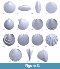
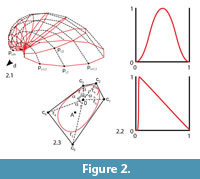Bivalve geometries were generated using a simple method similar to the ones mentioned in the introduction (Fowler et al., 1992). A planar closed aperture curve was defined using NURBS (non-uniform rational B-splines) and discretized into n aperture points (Figure 2). In m – 1 discrete growth steps, the aperture points were scaled by a scaling factor 1/λ < 1 and rotated around a fixed three-dimensional axis d lying in the same plane as the aperture curve. λ determined the inflation of the shell. A value of 1 would lead to a torus, slightly larger values to inflated shells and large values to very flat shells (cf. Figure 3.4–5). Instead of starting at the umbo, we created the desired final aperture curve and generated the shell backwards toward the umbo, in reverse biological growth direction:

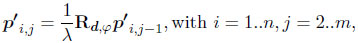
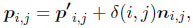
where p'_i,j is the three-dimensional surface point i of growth step j, λis the scaling factor and R_d,φ the 3×3 rotation matrix around the rotation axis d by angle φ. The points p'_i,1 were initialized by the aperture curve. The points p'_i,m constituted the umbo.

The surface sculpture was added in a second step by perturbing the surface in normal direction according to a scalar sculpture function δ(i, j) ∈ [0, 1]:

where the points p_i,j are the final three-dimensional surface points including surface sculpture and n_i,j is the normal vector at point p'_i,j. We used a sculpture function of the following structure:

where a ∈ [0, 1] is an overall sculpture amplitude parameter, w(j) is the maximal width or wavelength of a ridge (radial or commarginal) at the ventral edge at growth step j, q ∈[0, 1] is a parameter balancing radial and commarginal ridges, the functions δ_r, δ_c: [0, 1] → [0, 1] are the radial and commarginal profile curve, respectively, and f_r and f_c are frequency parameters determining how many radial and commarginal ridges, respectively, should be distributed over the whole shell. The parameter q allowed a gradual mixture of the sculpture from its radial and commarginal components. A value of 0 led to purely commarginal ridges, 1 to purely radial ridges. A value of 0.5 led to a mixture of equal parts of radial and commarginal ridges, i.e., a rectangular pattern. For a high flexibility in defining the profile curves δ_r and δ_cfor the ridges, again NURBS were used. For the evolutionary experiment, we used a symmetric smooth function with one peak for radial ridges and a jig-saw-shaped profile for commarginal ridges, as shown in Figure 2.2.

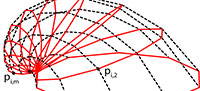
The result was a tube-like surface defined by n × m points p_i,j(Figure 2.1). To get a closed printable mesh, the small end forming the umbo was closed by a simple disc, while the large end forming the aperture and shell edge was closed by a flat disc featuring a bayonet coupling cavity for easy attachment to the other parts (see Figure 1.3).

We used a resolution of n = 400 by m = 720 and a rotation angle φ = 0.25° per growth step. This led to a valve covering 719 × 0.25° ≈ 180° or half a whorl. We stopped there, because the shells tapered fast towards the umbo and after 180° would cross the aperture plane, bending into the space occupied by the other valve.

To perform the morphological evolution experiments, we defined the aperture by a NURBS curve of order 4 with five control points c_k,, k = 1...5 (Figure 2.3). To define the shape of an aperture curve it would be possible to give the Cartesian (x, y)-coordinates of its control points. However, a continuous change of these coordinates would not lead to "natural" changes in the aperture curve. We therefore decoupled changes in tangential (commarginal) and radial direction by using polar coordinates instead of Cartesian coordinates. Two control points were summarized in one hinge segment. The aperture curve was therefore defined using four pairs of polar (r, α)-coordinates. The hinge angle α_h defined the angle between the two first control points, the hinge radius r_h the distance of both points to the origin. The aperture curve was aligned such that the hinge axis, i.e., the line through the first two control points, was parallel to the rotation axis d and the origin touching the discretized aperture curve. This ensured compact and printable geometries but allowed orthogyrate shells only (see also Future Work). The angle of the full circle not occupied by the hinge was partitioned into three sectors according to the three remaining control point angles α₃–α₅.

Since natural bivalve shells are often tilted towards anterior when burrowing, we introduced an angle parameter ϑ ∈ [0°, 90°] to determine this rotation. It ranged from 0°, where the hinge axis was horizontal and the umbo at the top, to 90°, where the anterior part of the shell pointed downwards and the hinge axis was vertical. Technically, this parameter rotated the bayonet coupling at the inside of the valves such that they were rotated relative to the central disc. The coupling structure was generated using computer-aided design (CAD) and was always placed at the incircle centre of the aperture curve.

As the purpose of this study was to investigate the shell shape, the volume of the shells was held constant. All shells were scaled such that the volume of one valve was 25 cm³.

Table 1 shows a complete list of the 14 parameters used to generate the shells. Since the parameters span a morphospace, we may call them morphological parameters. However, they do also represent a genotype, which is, using a virtual growth process, translated into a shell geometry, i.e., a phenotype. We therefore also call them genetic parameters. Figure 3 shows a set of sample shells illustrating how the genetic parameters affect the final shell shape.

Evolutionary Algorithm

Bivalve shell morphologies as defined above were subjected to an artificial evolutionary process in a series of experiments. Following the common terminology for evolutionary algorithms, we use the terms "genome" and "genetic" in an abstract sense to refer to a set of parameters defining the properties of an individual (in our case a bivalve shell morphology). This section explains how the parameters were encoded in an artificial genome, how that genome was adapted during evolution and how the experiments were performed.

Genome encoding. The genome consisted of 15 real numbers ∈ [0, 1]; the first 14 were mapped to the genetic parameters shown in Table 1, the last one encoded a mutation rate, see Evolution strategy. The values from the genome were directly used or linearly scaled to the appropriate range except for λ.

Shell inflation is a highly non-linear function of λ. To ensure a smooth linear change of the morphology as a response to a change in the genome, we therefore used a special mapping in this case. The value on the genome was used to encode the ratio of the width of one valve (distance from the aperture plane to the most distant point on the umbo) and the height (dorsal-ventral diameter of the aperture curve). This ratio was limited to [0.04, 0.39]. A value of 1 would imply a torus (and λ = 1). The value of λwas then determined such that the shell satisfied the given ratio.

To maintain an order of increasing angles for the control points c₃ to c₅, the corresponding parameter pairs (r₃, α₃)–(r₅, α₅) were first sorted according to the angle and then assigned to the control points in ascending order (i.e., the indices 3–5 of the control points and the parameter pairs may not match).

Despite the considerations above to find a natural encoding, it was still necessary to specifically test for invalid shells, i.e., shells that were not printable because their surface was self-intersecting or had too thin features. We employed the following criteria to detect invalid shells: a) crossing segments of the control polygon; b) an aperture with an incircle smaller than the metal disc (diameter 50 mm); c) an outside shell surface intersecting the inner attachment structure; d) a length-height ratio ∉ [1/5, 5]; and e) angles between segments of the control polygon below 10°, leading to too thin structures.

Fitness function. For each shell morphology, a fitness value was computed from the experimental results. It was used to measure the ability of the shell to vanish and hide below the sediment surface. We computed the fitness value F based on the final burrowing depth, as a sum of two volumes, F = V_b + V_c, where V_b was the part of the volume of one valve buried below the sediment surface and V_c was a virtual volume of sediment covering a completely buried shell.

For partially buried shells, V_c was 0. For completely buried shells (where V_b was equal to the full valve volume), V_c was computed as V_c= dA, where d was the distance of the top of the shell to the sediment surface and A was the average cross section of a valve with volume 25 cm³, i.e., . A fitness value of 0–25000 mm³ did therefore signify partial burial, while each additional 855 mm³ meant one more millimetre below sediment surface.

Both values, V_b and V_c, were computed from the burrowing depth measured by the linear motors. From the initial position and orientation of the shell, touching the sediment surface, and the displacement of both sliders, a final position and orientation of the shell was computed, assuming that the shell was moving in its sagittal plane and that the disc centre stayed in the same vertical line. These are reasonable assumptions due to the convergent nature of pulling motions. Visual observations of the final state of the shells at the end of the burrowing run were in accordance with the computed results. The main reason to compute the fitness value of a shell from the volumes V_b and V_c– rather than directly using the burrowing depth – was to avoid pathological cases such as shells with long thin ventral spikes. Using these, a shell could have just "fallen over" to get a high fitness, i.e., move down by rotating away the spike without actually entering the sediment.

Evolution strategy. A (2+3) evolution strategy (ES) was used for the experiments (Schwefel, 1995). This means that from a generation of shell morphologies, two were selected, which then produced three child morphologies; from all five morphologies, again two were selected for the next generation. We used a "+"-strategy as opposed to a ","-strategy (i.e., applied selection to the offspring and parents instead of only to the offspring, Schwefel, 1995), because we wanted to avoid the risk of losing good morphologies. The number of children was limited to three because of the size of the 3D printer; six was usually the maximum number of valves of the given volume that could be printed by the 3D printer in one job. Considering the long printing times (see Results), it was decided to set the offspring size accordingly.

From the full population of five different shell morphologies, the two with the highest fitness values were chosen. This kind of selection operator is called elitism and commonly used in evolutionary algorithms.

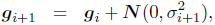
The reproduction operators were mutation and uniform crossover. Each of the two parents was mutated and a third child was generated by crossover + mutation. A self-adaptation scheme was used for the mutation rate (Beyer and Schwefel, 2002; Schwefel, 1995). Each genome g_i of generation i stored a value σ_i as its mutation rate. The mutated genome was then generated as follows:

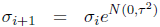
where is a scalar normally distributed around 0 with variance τ² and is a vector of length 14 of values normally distributed around 0 with variance . First, the mutation rate itself was changed using the parameter τ, then the rest of the genome was mutated using the new mutation rate. The genomes of the first generation g₁ were initialized randomly with values uniformly distributed in [0, 1]. As an initial mutation rate, we set σ₁ = 0.1 for all genomes. For τwe used a value of 1. This is higher than the standard value of 0.3 proposed by the literature (Beyer, 1995), because we decided to allow for a faster adaptation of the mutation rate due to the small number of children and generations.

Uniform crossover was done by randomly and independently choosing each value of the genome either from the first or second parent, with equal probability (Gilbert Syswerda, 1989). Because we could only perform a small number of generations, it was important to be able to combine successful traits of different individuals.

As explained in Genome encoding, some genomes led to invalid shell geometries. During the reproduction phase, we therefore discarded any invalid morphology and generated new genomes until one was valid. This led to an artificial reduction of the mutation rate, as the probability to be valid was higher for offspring close to the valid parent. To counteract this effect, we generated three versions of each generation and chose the one with the highest diversity.

Experiments. For the experiments, the following steps were repeated for each generation: 1. print the three new shells, 2. evaluate them and re-evaluate the two individuals selected from the last generation, 3. from the five shells, select the two with the highest fitness, 4. use them to generate three new shells by mutation and crossover.

Before each burrowing run, the sediment was treated to establish a standardized configuration. This was done by manually pressing a small metal plate on the sediment surface to increase its compaction and to undo the loosening caused by retrieving the shell from the previous burrowing run. The height and planarity of the sediment surface was ensured by sliding a metal strip over two metal bars horizontally fixed to either side of the sediment compartment. As explained in Limitations, we could not avoid a memory effect of the sediment, i.e., a dependence of the sediment state on earlier experiments. Usually, the sediment became more compacted in the course of the experiments.

To deal with the fluctuations in the sediment, each burrowing run was repeated 10 times. The fitness value for a morphology was therefore based on 10 successive evaluations of the shell. Also, already evaluated and selected parent individuals were re-evaluated in each generation.

To evaluate the different morphologies, only the valves were exchanged, the central metal disc and all other parts of the setup were re-used for all experiments. The computer program did not only execute the evolution strategy and generate the new shell morphologies but did also automatically adapt the control programs of the linear motors. To ensure a consistent initial position of the different shell morphologies, touching the sediment surface, it was necessary to adjust the initial position of the sliders.

Phenotypic Parameters

In addition to the genetic (or morphological) parameters used to generate the shells, we computed a set of derived phenotypic (or morphometric) parameters to describe the shell morphology in more detail and to test for correlations with the fitness. Because the exact geometries of all shells were known, the phenotypic parameters could be computed exactly as well. Table 2 shows a list of the derived parameters. Note that the evolutionary algorithm modified the genetic parameters, while the phenotypic parameters were computed afterwards from the resulting shell geometries.

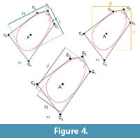Length L, height H and width W are the standard shell dimensions used in biology. Since we allowed the shell to rotate towards anterior by adding the parameter ϑ, the two dimensions L and H may rotate with respect to the environment. We therefore introduced measures perpendicular to the coordinate system of the environment. The tallness T measured the shell dimension along the burrowing direction, i.e., perpendicular to the sediment surface. The broadness B measured the dimension perpendicular to T, i.e., parallel to the sediment surface. Finally, we also computed the largest overall dimension J of the shell and the dimension parallel to it, N. All these additional measures lay in the sagittal plane of the shell, while the third direction was always measured by W (which in our case covered both valves and the central metal disc). See Figure 4 for an illustration of the different dimensions.

The other morphometric measures included the length l_A and area A_A of the aperture curve and the ratio γ= (A_c– A_A)/A_c, where A_c is the area of the convex hull of the aperture curve. If γis 0, the aperture curve itself is convex, the higher γ becomes, the more indentations there are in the aperture curve, leading to ears as in Figure 3.6, or shells with more than one spine. We also computed the relative positions of the umbo (average of all surface points p_i,m, i = 1..n) and the centre (of the incircle of the aperture curve, where the attachment structure was placed) and three different measures of streamlining.

Streamlining is a value assessing the average alignment of the shell surface with the burrowing direction. Shapes with a large flat area opposing (perpendicular to) the burrowing motion have values close to 0, while shapes with a small front but a large lateral area have values close to 1. Because it is difficult to compute an exact value from given natural bivalve shells, Watters (1993) defined an approximation for streamlining as

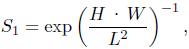
where H, W and L are height, width and length, respectively, as defined in Table 2. For the formula, Watters assumed the length to be the dimension in burrowing direction. Since in our case, we actually know the burrowing direction for each shell, we can define a second measure of streamlining, S₂ using the same formula but computed from broadness B, width W and tallness T, instead of H, W and L, respectively.

Since we knew both the orientation of the shells with respect to the burrowing direction and the shell geometry, it was possible to compute an exact measure of streamlining, S₃. The angles between the shell mesh faces (the rectangular facets in Figure 2.1) and the burrowing direction were scaled to [0, 1] (with 0 = perpendicular to the burrowing direction and 1 = parallel to the burrowing direction), weighted using the corresponding face areas and aggregated to compute an average. Very flat shells (small W) tended to have values close to 1, while highly inflated shells tended to have values close to 0.5. Values close to 0 were not possible with our geometric model.

RESULTS

Using the described setup and evolution strategy, 20 generations of artificial evolution were performed. The number of printed shells was 60. On average, one generation needed a printing time of 20 h and 139 cm³ of printing material.

Burrowing Depth, Fitness and Sediment

Figure 5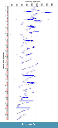 shows the burrowing depths that were measured during the course of the evolution. They continuously decreased by about 14 mm over the 20 generations. In an evolutionary experiment, it should be expected that fitness, which in our experiments was indirectly linked to the burrowing depth, increases during the course of evolution. In the case of a "+"-strategy it is even guaranteed that the best fitness does not decrease from generation to generation, provided the same individual is always mapped to the same fitness value. This requirement is not met in cases where the fitness value is based on a physical measurement. In this study, fitness did not only depend on the morphology but also on the state of the sediment. From previous experiments (Germann and Carbajal, 2013), we know that the state of the sediment has a large influence on the burrowing process, see also Limitations. There was a memory effect, i.e., a burrowing run was not independent of previous burrowing runs. Over the period of several experiments, the compaction of the sediment usually increased continuously. This counteracted the effect of more adapted shell morphologies that evolved.

The variance of the burrowing depth within the 10 repetitions of an evaluation is in most cases small enough to allow comparisons in burrowing performance. Outliers or large variances can usually be explained by accidents like connectors that broke loose from the shell and that had to be retrieved from within the sediment (e.g., shell 1 in generation 3 or shell 47 in generation 17). When testing the differences between the five individuals within a generation using a Wilcoxon ranksum test at a 0.05 confidence level, 81% of all differences are significant. However, we cannot reliably determine how much of this difference is indeed caused by the shell morphology and how much by fluctuations in the state of the sediment.

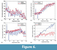Because of the sediment fluctuations we re-evaluated selected shells in each generation. In the ideal case, morphology would be the only factor influencing the burrowing depth, and the re-evaluated individuals would reach exactly the same depth as in all previous evaluations. Figure 6.1 shows a plot of all burrowing depths, with identified repetitions. It is possible to compute a correction vector that shifts the data points vertically to make the repetitions match. However, there is no unique solution, so although such a correction vector helps to correct the repetitions, it cannot reveal the true global course of the curve, i.e., the curve we would have gotten if we could return the sediment in the exact same state before each burrowing run. In Figure 6.2-3, we show two solutions for a correction. For the first correction, "shift 1," we computed a shift vector for each repeated individual that assumed that the shift value for the last repetition stayed the same for the following experiments (i.e., that the compaction of the sediment up to this point in time was irreversible). This led to a strongly increasing depth curve shown in Figure 6.2. For the alternative correction "shift 2" shown in Figure 6.3, the shift vector was adjusted such that the linear regression line through the resulting depth curve was horizontal. The shift vectors for both types of correction are shown in Figure 6.4.

Figure 7.1 shows 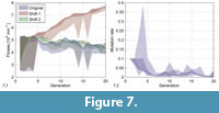a comparison of the original fitness values and two versions corrected using an analogous method as for the depth. The fitness values of the different individuals are summarized by areas covering all (bright area) and only the selected individuals (dark area). According to our experience with the behaviour of the sediment, we suspect that the curve would lie between the two corrections, but closer to the shift 2 correction, if we could perform experiments with a perfectly standardized sediment. In the rest of this section, we therefore show results based on the original data or of the shift 2 correction.

Figure 7.2 shows the same kind of range evolution plot for the mutation rate. It decreased quickly from the initial value of 0.1 and then fluctuated around a tenth of this value.

Phylogeny

Figure 8 shows the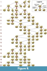 complete phylogenetic tree of the evolutionary experiment. The number of occurrences of the two types of reproduction, mutation and crossover + mutation, does not indicate any advantage of one over the other. In the fittest individuals, the ratio is 7:5, in the selected individuals 16:8, i.e., the ratios do not deviate from the overall ratio of 2:1. Among selected individuals, crossover was mainly present in generations 7–13.

All individuals from generation 3 onwards were descendants of shell 1. Together with the decreasing mutation rate, this led to a high similarity among the shells of the remaining generations. While the shell shape moderately changed towards taller shells and back to shells with a lower tallness, the shell sculpture basically stayed constant, featuring commarginal ridges of an intermediate frequency and amplitude.

The comparison of different shells reveals the important role of tallness. Based on the original data, shell 58 was the best shell of the final generation (see Figure 8). Overall, shell 10 in generation 4 was the best (fittest) individual, followed by shell 1 in generation 2. All of these shells had a low or moderate tallness. Shell 5 in generation 2 was the worst individual, followed by shell 9. These were also the tallest shells. Shell 6 had the greatest burrowing depth but was very tall, which led to a low fitness. These rankings are similar but not identical in the corrected versions of the data.

Correlation of Parameters with Fitness

Because the rotation angle ϑwas virtually always close to 90° and most shells had their largest diameter perpendicular to the hinge axis, the dimension measures strongly correlate. Length correlates (Pearson) with tallness by r = 0.92 (p-value = 2×10^–25) and with the major axis length by r = 0.55 (p-value = 7×10^–6). Height correlates with broadness by r = 0.90 (p-value = 3×10^–22) and with the major axis length by r = 0.34 (p-value = 0.008). While the major and minor axes are sometimes misaligned, length is basically equivalent to tallness and height to broadness. Figure 4 shows the measures for individual 6, which is an exception in the sense that the measures do not align.

Figure 9 shows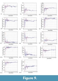 the evolution of the genetic parameters over the generations. After a quick convergence during the first three to five generations, most values stayed virtually constant. Some parameters show a slight change around generation 15. It can be seen that the parameter values of invalid shells cover a larger interval than those of valid shells.

To investigate the distribution of invalid shells, we generated a sample of 10000 random individuals. Fourteen percent of these were valid, while in the evolutionary experiment, 56% of the generated shells were valid. In the sample, the valid shells were evenly distributed throughout the parameter space except for λ, r_h and the angles α₃-α₅. Valid shells were restricted to an interval of about [0.1, 0.8] in λ. Also, there were more valid shells for higher values of r_h. There were less valid shells in the regions where two of the angles α₃-α₅ had a similar value.

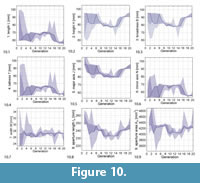
Figure 10 shows how the computed phenotypic parameters changed over the course of evolution.

Correlations of the genetic and the phenotypic parameters and the burrowing depth D with the fitness are listed in Table 3. The table is sorted according to the p-value of the Pearson correlation. The order is similar for the original fitness measure and the one corrected by "shift 2." The shift 2 correction of the fitness values often increases the correlation coefficients, e.g., from -0.68 to -0.73 for the tallness.

DISCUSSION

In this paper we presented an experimental setup to simulate the burrowing behaviour and morphological evolution of bivalves. Using evolutionary algorithms, the first ever artificially evolved bivalve shapes were created. While the used method as such has many advantages, the system suffered from two main drawbacks. Because of the lack of an optimal mechanism to standardize the sediment, fluctuations in the sediment state disturbed the performance measure of the different individuals. And due to geometrical restrictions of the valves used to assemble the shells, many created geometries were invalid, increasing the brittleness of the evolutionary system.

Evolution Results

As seen in Figure 5, depth decreased during the course of the evolutionary experiments. The difference between the median depth in the first generation and the median depth in the last generation is 13.8 mm. As the fitness and with it the burrowing depth would be expected to increase during evolution, it can be assumed that this difference is due to the increasing compaction of the sediment. A similar value is observed in the repeated evaluations of individuals in Figure 6.1. The maximal range of different measurements for one single individual is 16.8 mm.

In contrast, the difference between all possible pairs within all generations is 5.1 mm ± 3.6 mm (mean ± standard deviation). Therefore, the influence of the sediment by far overweighs the effect of the shell morphology. This indicates that there may be a large pressure on bivalves to manipulate the sediment state, which they actually do by expelling water and moving the foot and the valves.

In this study, however, we were only concerned with the influence of the shell morphology on the burrowing performance. Although the repeated evaluations of individual shells gave a hint at how the state of the sediment changed, they did not suffice to remove the noise of the sediment. We therefore do not know the true depth curve, i.e., the depths that would have resulted if the sediment could be put into an identical state before each burrowing run.

The burrowing depth and indirectly the shell tallness were the two basic components of the fitness. This fact is reflected by the high correlation of the depths D minus tallness T with fitness shown in Table 3. The next highest correlations were found for tallness and length, which basically mean the same. A lower tallness improves the ability of the shell to vanish below the sediment surface and thus increases the fitness. While the burrowing depth decreased over the course of evolution due to the increasing sediment compaction, tallness may have been the main variable for evolution to optimize. This is supported by the fact that the correlation between tallness T and fitness is much higher than between burrowing depth D and fitness.

Also, tallness had a larger variance than the burrowing depth: the overall burrowing depth was 95.6 mm ± 5.9 mm (mean ± standard deviation), i.e., varied by 6.2%, the overall tallness was 65.1 mm ± 10.5 mm varying by 16.2%. This indicates that it was easier to maximize fitness by a low tallness than by further penetrating into the sediment. The shell was therefore "spread" horizontally to occupy the top sediment layer where penetration was much easier than in deeper layers.

Since tallness was not controlled by one single parameter, the aperture curve had to be changed accordingly, involving eight aperture parameters as well as ϑand λ. The latter does not change the ratio of the dimensions but, via the constant volume, the absolute size of the dimensions. In our experiments, we may have had a trade-off for λbetween a small width W and a small tallness T. This may explain the low correlation of λ with fitness. For a fitness function only based on burrowing depth, we would probably have seen a significant decrease of W (increase of λ) over time.

Following tallness and length, streamlining S₂ had the next largest correlation with fitness. Note that the correlation coefficient of the streamlining S₃ has the opposite sign of that of S₂ and S₁. Fitness decreased with increasing streamlining S₂ but increased with increasing S₃. The assumption behind S₁ and S₂ is that streamlining grows with increasing vertical elongation of the shell and decreasing cross-sectional area perpendicular to the burrowing direction. However, the diverging results for the different measures show that the approximated value can be very different from a computation based on the actual shell geometry.

In our experiments, the effect of the overall shape was more important than the sculpture, which essentially stayed constant. There is only one sculpture parameter in the first half of Table 3, radial sculpture frequency f_r. However, since radial ridges were basically not expressed due to a low q parameter, it is likely that this parameter was coupled to another successful trait but did not increase fitness by itself. A reason for the low impact of the shell sculpture on fitness may also be that in our setup its function is limited to supporting the burrowing process. Most sculptural elements of the shell are interpreted as barbs (Seilacher, 1981). Their function is to reduce the buoyancy of the shell during the digging. In our experimental setting, the steel cables simulating the pulling force of the foot muscles are under tension during the entire experiment and thus prevent the shell from floating up.

The fitness curve (Figure 7.1) did not feature major jumps, i.e., there was no instance of an innovative morphological feature significantly increasing fitness. As long as shell 1 stayed in the population, it produced a set of distinct shell morphologies (shells 4, 6, 9 and 11, see Figure 8), which, however, had all a low fitness. Later shells were all very similar due to the decreased mutation rate. More differing shells like 42 and 46 were penalized with a low fitness (drops in generations 14 and 16 in Figure 7.1).

As can be seen in the genetic parameter range evolution plot (Figure 9), the range of possible values was not covered and the values stayed relatively stable during the whole evolution. The phenotypic parameter range evolution plot (Figure 10) shows that there were still two minor transitions, separating the evolution into three phases, at generations 5–7 and 14–16. In the middle phase, shells were relatively tall, returning to a low tallness in the transition to the third phase.

Compared to the realized parameters, the parameters that were tried but resulted in invalid shells covered a larger interval (Figure 9). This indicates that invalidity may account for the stability of the values during evolution. Because the probability of hitting a valid shell was larger close to an already realized valid shell, evolution reduced the mutation rate leading to a stagnating pool of shell morphologies. The procedure of generating three new generations and choosing the one with the largest variation did not suffice to counteract this effect.

To summarize, our experiments led to a clear ranking of factors in terms of the effect size on burrowing performance: 1. sediment state, 2. overall shape, 3. sculpture. It is interesting to note that in both our experiment and in nature, elongated shells evolved (Kauffman, 1969). However, in our experiments, due to the restriction to a rigid morphology, there was an evolutionary pressure for elongation in horizontal direction to avoid deeper and harder layers of sediment. In nature, bivalves can take advantage of water ejection and valve motion to manipulate the sediment state, which enables them to reach deeper layers and makes an elongation in burrowing direction more beneficial.

Limitations

No biomimetic setup is able to imitate all aspects of the original process in nature. The impact of the experiments depends on how well the setup manages to simulate the components essential to the research question. In this study we examined the influence of the shell morphology on burrowing performance in bivalves using a rocking burrowing motion. Some aspects of bivalve burrowing were omitted, e.g., water expulsion.

The major limitation of the presented setup was the lack of an effective method to standardize the sediment before each burrowing run. Pressing a metal plate onto the sediment did not provide a satisfactory reduction of the memory effect. The noise thus introduced into the fitness reduces the comparability of different morphologies because the effect of the sediment cannot be clearly separated from the effect of the morphology. Since the differences between individuals usually decrease during evolution, the result of selection will be increasingly random.

Brittleness is the probability that a small change in the parameters will have a large effect on the fitness, e.g., lead to a sharp drop in fitness or even to an invalid individual that cannot be evaluated (Ronald, 1997). In the applied evolutionary algorithm, the major drawback was the increased brittleness due to invalid shells. Small changes in the parameters were able to render a well performing shell invalid. Still, we found that shells closer to a valid shell were more likely to be valid as well. This led to a fast decrease in the adaptive mutation rate. To counteract this effect, we employed a mechanism that generated three versions of a new generation and then manually chose the one with the highest variety. This whole procedure is not satisfactory. For future experiments, the morphological shell model, its encoding and the geometrical restrictions due to the coupling mechanism should therefore be revised to avoid invalid shells.

According to Arnold (1983), the mapping from morphology to fitness can be separated into the mapping from morphology to performance and the mapping from performance to fitness. Our study is based on two simplifying assumptions or restrictions that need to be considered when interpreting the results: 1) it is assumed that there is only one performance variable, namely burrowing performance; and 2) it is assumed that fitness is proportional to burrowing performance.

Both assumptions are not generally true. The shell morphology does, e.g., also influence the overall fitness by its performance in anchoring within the sediment or in protection against predators. Also, it is not entirely clear if there is an evolutionary pressure to go as deep into the sediment as possible, since several other factors like the concentration of oxygen or nutrients influence burrowing depth as well (da Silva Cândido and Brazil Romero, 2007; Edelaar, 2000; Marsden and Bressington, 2009; Schwalb and Pusch, 2007; Stanley, 1970). We assume that there is nevertheless a pressure to hide the shell within the sediment by at least burying the whole shell, and that therefore it is reasonable to assume a linear relationship between burrowing performance and fitness in the depth ranges covered in this study. While the two assumptions restrict the generality of the reported results, they help focus on a practicable and relevant subset of the natural phenomenon.

Another drawback of the experiments is the large required effort in time and resources. As a result, only a small population and a small number of generations could be simulated. This increases the probability to get stuck in local optima of the fitness landscape.

Future Work

The experiments in this study may be repeated under both the same and different conditions (esp. fitness function, initial population) to get a better understanding of general evolutionary pressures working on the functional morphology of burrowing bivalves. To perform efficient experiments, the execution of repeated burrowing runs should be automated.

Any study trying to repeat experiments of a similar kind as described here should implement an improved method to standardize the sediment between burrowing runs. We suggest using a combination of sediment loosening, e.g., by a high pressure water supply in the bottom plate, and subsequent uniform sediment compaction, e.g., by vibrating the whole sediment compartment.

While in evolutionary robotics usually only the controller of a robot is evolved (Floreano et al., 2008), our setup can easily be used to co-evolve the shell morphology and burrowing motion pattern. It would be interesting to study the interaction of morphology and control in evolution.

The mathematical model of the shell morphology may be replaced or extended to capture a larger variety of overall shell shapes. In particular, the evolved shells were all orthogyrate, while many burrowing bivalve species have prosogyrate shells. This condition is known to be beneficial for burrowing (Stanley, 1975b).

The surface sculpture in this study was limited to radial and commarginal ridges and mixtures of them. Findings of Stanley (1969) suggest that skew ridges may improve the burrowing performance. To test this, a method that can generate a larger variety of surface patterns, including skew ridges, should be used. We would suggest to apply a reaction-diffusion system similar to the one described by Meinhardt and Klingler (1987).

The setup may be used to test the properties of fossil shapes. Using a computed tomography (CT) scanner, a fossil may be digitized and after the necessary modifications 3D printed as plastic valves. The shape could then be compared to other shapes, e.g., from recent related species. By testing the fossil shape in different types of sand, one could learn more about the possible habitats of the fossil species. Also, using artificial evolution, it may be possible to identify the most suitable burrowing motion for a given fossil.

CONCLUSION

To our knowledge, we were the first to perform an experiment to evolve physical bivalve shell morphologies using an evolutionary algorithm. We combined well established components like geometric models for generating bivalve shell shapes, evolutionary algorithms and 3D printing devices. The experiments were done in a tank containing water and sand, the rocking burrowing motion typical for bivalves was applied to the printed shells by an external actuation system.

The results show that the influence of the sediment state is a main – and so far underestimated – factor for the effectiveness of bivalve burrowing. Granular media show highly complex dynamics that are still not well understood (Jaeger and Nagel, 1992; Losert et al., 2000; Sassa et al., 2011; To et al., 2001; Umbanhowar and Goldman, 2010). As long as there are no reliable and detailed computer simulations available, only physical experiments can deliver realistic results. When just considering shell morphology and ignoring the influence of the valve and foot motion, shells with a small vertical diameter are best suited to vanish within the sediment, confirming the high resistance of deeper sediment layers and the necessity for the manipulation of the sediment compaction state to burrow deeper. Commarginal and radial shell sculpture plays a minor role in the effectiveness of burrowing, if we can exclude buoyancy.

While the synthetic approach is used in biomimetic projects to emulate a large variety of recent organisms and animal behaviour, it is not common in palaeontology. However, we suggest it is well suited to complement analytical studies, e.g., by testing the morphological features of fossil species in an experimental setup like the one presented here. Moreover, it is insightful to not only emulate the dynamics of behaviour, but also evolutionary pressure. This is the main idea of the described method. While evolutionary algorithms are commonly used as bio-inspired optimization techniques, we believe that the reverse way is just as fruitful: using them as a tool to identify and study evolutionary pressure on the functional morphology of organisms.

Evolutionary algorithms contrast to other models of evolution, common in palaeontology, which are based on statistics, population means and empirically determined rates of evolution (Arnold et al., 2002; Lande, 1976; Polly, 2004). While those approaches quantify evolutionary change by statistically analysing large data sets of phenotypic characters of natural species, the approach using evolutionary algorithms actively simulates the process of evolution and is based on an artificial genome that is used to generate different specific morphologies that are tested using a specific fitness function. We do not suggest to replace any method by the proposed method, but we believe it is a valuable additional tool that is particularly suited to test specific hypotheses and to generate and compare morphologies that do not exist in nature. A disadvantage of the proposed method may be that it is more difficult to relate the results to natural species and that only small population sizes and generation numbers are possible due to the resources and time needed to build the physical setup, to print the shells and to perform the experiments.

Although the presented setup had drawbacks, we believe that the method has a large potential for future studies. In particular, we see the following advantages of our method: 1) In addition to standard morphometric analyses of fossilized shapes, the functional morphology can be tested in action; 2) Tests are more realistic using a physical setup than a computer simulation, especially for sandy sediments that are still hard to simulate in the computer; 3) Factors that may have exerted an evolutionary pressure on functional morphology may be isolated; 4) Optimal burrowing morphologies can be generated under different conditions (fitness functions); 5) Using morphological models and 3D printers, the whole theoretical morphospace can be covered, there is no restriction to the shapes of available specimens; 6) Innovations in functional morphology can be identified by analysing jumps or other transitions in the artificial evolution; 7) The bivalve shell morphology and the applied burrowing motion pattern can be completely controlled, which allows systematic experiments or the application of evolutionary algorithms; 8) The burrowing performance can be quantified using different sensors; 9) Due to the full access to the detailed geometry of all shells, morphometric measures such as streamlining can be computed exactly; 10) The exact definition of the shell morphologies increases the repeatability of experiments; 11) several aspects of the method, like the mathematical shell model, the burrowing motion or the fitness function, can be easily changed to reflect the purpose of future experiments; 12) 3D printing techniques will be cheaper, faster, more accurate and possibly extend to other materials in the future and offer even more possibilities to investigate (functional) morphologies.

ACKNOWLEDGEMENTS

The authors would like to thank R. Pfeifer for providing the AILab infrastructure including the 3D printer. We would also like to thank the Swiss National Science Foundation for funding this research (projects 113934 and 129900).

REFERENCES

Adams, D.C., Rohlf, F.J., and Slice, D.E. 2004. Geometric morphometrics: Ten years of progress following the "revolution." Italian Journal of Zoology, 71:5–16.

Amler, M., Fischer, R., and Schröder-Rogalla, N. 2000. Muscheln, volume 5 of Haeckel-Bücherei. Enke im Georg Thieme-Verlag, Stuttgart.

Arnold, S., Pfrender, M., and Jones, A. 2002. The adaptive landscape as a conceptual bridge between micro- and macroevolution. In Hendry, A. and Kinnison, M. (eds.), Microevolution Rate, Pattern, Process, volume 8 of Contemporary Issues in Genetics and Evolution, pp. 9–32. Springer Netherlands. doi: 10.1007/978-94-010-0585-2_ 2.

Arnold, S.J. 1983. Morphology, performance and fitness. Integrative and Comparative Biology, 23:347–361. doi:10.1093/icb/23. 2.347.

Bäck, T. 1997. Handbook of Evolutionary Computation. Oxford University Press, New York.

Bentley, P.J. 1999. Evolutionary Design by Computers. Morgan Kaufmann Publishers, San Francisco, CA.

Beyer, H.G. 1995. Toward a theory of evolution strategies: Self-adaptation. Evolutionary Computation, 3:311–347. doi:10.1162/ evco.1995.3.3.311.

Beyer, H.G. and Schwefel, H.P. 2002. Evolution strategies – a comprehensive introduction. Natural Computing, 1:3–52. doi:10.1023/A:1015059928466.

Bookstein, F.L. 1997. Morphometric Tools for Landmark Data: Geometry and Biology. Repr. edition. Cambridge University Press, Cambridge.

Crampton, J.S. 1995. Elliptic fourier shape analysis of fossil bivalves: some practical considerations. Lethaia, 28:179–186. doi: 10.1111/j.1502-3931.1995.tb01611.x.

da Silva Cândido, L.T. and Brazil Romero, S.M. 2007. A contribution to the knowledge of the behaviour of anodontites trapesialis (bivalvia: Mycetopodidae). The effect of sediment type on burrowing. Belgian Journal of Zoology, 137:11–16.

de la Huz, R., Lastra, M., and López, J. 2002. The influence of sediment grain size on burrowing, growth and metabolism of donax trunculus l. (Bivalvia: Donacidae). Journal of Sea Research, 47:85–95. doi: 10.1016/S1385-1101(02)00108-9.

Dryden, I.L. and Mardia, K. 1998. Statistical Shape Analysis. Wiley series in probability and statistics. Wiley & Sons, Chichester.

Edelaar, P. 2000. Phenotypic plasticity of burrowing depth in the bivalve Macoma balthica: experimental evidence and general implications. Evolutionary biology of the Bivalvia, 177:451–458.

Eggenberger Hotz, P. 2003. Genome-physics interaction as a new concept to reduce the number of genetic parameters in artificial evolution. In IEEE Congress on Evolutionary Computation, CEC '03, pp. 191–198. IEEE. doi: 10.1109/CEC.2003.1299574.

Floreano, D., Husbands, P., and Nolfi, S. 2008. Evolutionary robotics. In Siciliano, B. and Khatib, O. (eds.), Springer Handbook of Robotics. Springer, Berlin.

Fogel, D.B. 1998. Evolutionary Computation: The Fossil Record. 1 edition. Wiley-IEEE Press.

Fowler, D.R., Meinhardt, H., and Prusinkiewicz, P. 1992. Modeling seashells. In Catmull, E.E. and McCormick, B.H. (eds.), SIGGRAPH '92 conference proceedings, volume 26.1992,2 of Computer graphics, pp. 379–387. ACM Press, New York.

Germann, D.P. and Carbajal, J.P. 2013. Burrowing behaviour of robotic bivalves with synthetic morphologies. Bioinspiration & Biomimetics, 8:046009. doi: 10.1088/1748-3182/8/4/046009.

Hammer, Ø. and Bucher, H. 2005. Models for the morphogenesis of the molluscan shell. Lethaia, 38:111–122.

Jaeger, H.M. and Nagel, S.R. 1992. Physics of the granular state. Science, 255:1523–1531. doi: 10.1126/science.255.5051.1523.

Kauffman, E.G., 1969. Form, function, and evolution. In Cox, L.R. (ed.), Mollusca 6: Bivalvia, Treatise on invertebrate paleontology Part N N 0028639. The Geological Society of America.

Koller-Hodac, A., Germann, D.P., Gilgen, A., Dietrich, K., Hadorn, M., Schatz, W., and Eggenberger Hotz, P. 2010. Actuated bivalve robot: Study of the burrowing locomotion in sediment. In IEEE International Conference on Robotics and Automation (ICRA), 2010, pp. 1209–1214. IEEE, Piscataway, NJ.

Lande, R. 1976. Natural selection and random genetic drift in phenotypic evolution. Evolution, 30:314. doi: 10.2307/2407703.

Langton, C.G. 1989. Artificial life: The proceedings of an Interdisciplinary Workshop on the Synthesis and Simulation of Living Systems held September, 1987, in Los Alamos, New Mexico, volume 6 of Santa Fe Institute Studies in the Sciences of Complexity. Proceedings. Addison-Wesley, Redwood City Calif.

Lipson, H. and Pollack, J.B. 2000. Automatic design and manufacture of robotic lifeforms. Nature, 406:974–978.

Losert, W., Géminard, J.C., Nasuno, S., and Gollub, J. 2000. Mechanisms for slow strengthening in granular materials. Physical Review E, 61:4060–4068.

Marsden, I.D. and Bressington, M.J. 2009. Effects of macroalgal mats and hypoxia on burrowing depth of the new zealand cockle (Austrovenus stutchburyi). Estuarine, Coastal and Shelf Science, 81:438–444. doi:10.1016/j.ecss.2008.11.022.

McGhee, G.R. 1999. Theoretical Morphology: The Concept and Its Applications. Perspectives in paleobiology and earth history. Columbia University Press, New York, USA.

Meinhardt, H. and Klingler, M. 1987. A model for pattern formation on the shells of molluscs. Journal of Theoretical Biology, 126:63–89.

Okamoto, T. 1988. Analysis of heteromorph ammonoids by differential geometry. Palaeontology, 31:35–52.

Polly, P.D. 2004. On the simulation of the evolution of morphological shape: multivariate shape under selection and drift. Palaeontologia Electronica, Vol. 7, Issue 2; 7A:28pp.
palaeo-electronica.org/2004_2/evo/issue2_04.htm

Raup, D.M. and Michelson, A. 1965. Theoretical morphology of the coiled shell. Science, 147:1294–1295. 10.1126/science.147. 3663.1294.

Rechenberg, I. 1973. Evolutionsstrategie: Optimierung technischer Systeme nach Prinzipien der biologischen Evolution, volume 15 of Problemata. Frommann-Holzboog, Stuttgart-Bad Cannstatt.

Rechenberg, I. 2000. Case studies in evolutionary experimentation and computation. Computer Methods in Applied Mechanics and Engineering, 186:125–140. doi: 10.1016/S0045-7825(99)00381-3.

Ronald, S. 1997. Robust encodings in genetic algorithms: a survey of encoding issues. In Proceedings of 1997 IEEE International Conference on Evolutionary Computation (ICEC '97), pp. 43–48. IEEE. doi:10.1109/ICEC.1997.592265.

Sassa, S., Watabe, Y., Yang, S., Kuwae, T., and Thrush, S. 2011. Burrowing criteria and burrowing mode adjustment in bivalves to varying geoenvironmental conditions in intertidal flats and beaches. PLoS ONE, 6:e25041. doi: 10.1371/journal.pone.0025041.

Savazzi, E. and Huazhang, P.A. 1994. Experiments on the frictional properties of terrace sculptures. Lethaia, 27:325–336. doi: 10.1111/j.1502-3931.1994.tb01583.x.

Schwalb, A.N. and Pusch, M.T. 2007. Horizontal and vertical movements of unionid mussels in a lowland river. Journal of the North American Benthological Society, 26:261–272. doi: 10.1899/ 0887-3593(2007)26[261:HAVMOU]2.0.CO;2.

Schwefel, H.P. 1995. Evolution and Optimum Seeking. Sixth-generation computer technology series. Wiley, New York.

Seilacher, A. 1981. Konstruktionsmorphologie von Muschelgehäusen. In W.E. Reif (ed.), Funktionsmorphologie, Paläontologische Kursbücher Band 1. Paläontologische Gesellschaft.

Seilacher, A. 1984. Constructional morphology of bivalves: Evolutionary pathways in primary versus secondary soft-bottom dwellers. Palaeontology, 27:207–237.

Sims, K. 1994. Evolving 3d morphology and behavior by competition. Artificial Life, 1:353–372. doi:10.1162/artl.1994.1.4.353.

Stanley, S.M. 1968. Post-paleozoic adaptive radiation of infaunal bivalve molluscs: A consequence of mantle fusion and siphon formation. Journal of Paleontology, 42:214–229.

Stanley, S.M. 1969. Bivalve mollusk burrowing aided by discordant shell ornamentation. Science, 166:634–635. 10.1126/ science.166.3905.634.

Stanley, S.M. 1970. Relation of shell form to life habits of the Bivalvia (Mollusca), volume 125 of Memoir / The Geological Society of America. The Geological Society of America, Boulder, Colorado, USA.

Stanley, S.M. 1975a. Adaptive themes in the evolution of the Bivalvia (mollusca). Annual Review of Earth and Planetary Sciences, 3:361–385. doi:0.1146/annurev.ea.03.050175.002045.

Stanley, S.M. 1975b. Why clams have the shape they have: An experimental analysis of burrowing. Paleobiology, 1:48–58.

Syswerda, G. 1989. Uniform crossover in genetic algorithms. In Schaffer, J.D. (ed.), Proceedings of the 3rd International Conference on Genetic Algorithms, George Mason University, Fairfax, Virginia, USA, June 1989, pp. 2–9. Morgan Kaufmann.

To, K., Lai, P.Y., and Pak, H. 2001. Jamming of granular flow in a two-dimensional hopper. Physical Review Letters, 86:71–74. doi: 10.1103/PhysRevLett.86.71.

Trueman, E.R. 1966. Bivalve mollusks: Fluid dynamics of burrowing. Science, 152:523–525. doi: 10.1126/science.152.3721.523.

Umbanhowar, P. and Goldman, D.I. 2010. Granular impact and the critical packing state. Physical Review E, 82. doi:10.1103/ PhysRevE.82.010301.

Watters, G.T. 1993. Some aspects of the functional morphology of the shell of infaunal bivalves (mollusca). Malacologia, 35:315–342.

Webb, B. 2000. What does robotics offer animal behaviour? Animal Behaviour, 60:545–558. doi:10.1006/anbe.2000.1514.

Winter, A.G., Deits, R.L.H., and Hosoi, A.E. 2012. Localized fluidization burrowing mechanics of ensis directus. Journal of Experimental Biology, 215:2072–2080. doi: 10.1242/jeb.058172.