Simulating abrupt change

Simulating our ability to accurately detect abrupt changes in assemblage-based paleoenvironmental proxies

Christina L. Belanger and David W. Bapst

Article number: 26.2.a24
https://doi.org/10.26879/1282
Copyright Paleontological Society, July 2023

Author biographies
Plain-language and multi-lingual abstracts
PDF version

Submission: 15 March 2023. Acceptance: 26 June 2023.

ABSTRACT

Resolving abrupt environmental changes in sedimentary records is critical to understanding environmental perturbations relevant on human timescales. The paleontological assemblage mixer (paleoAM) framework developed here simulates sedimentary records to measure the preservation potential of abrupt changes in assemblage-based faunal proxies while varying environmental background conditions, excursion magnitudes and durations, bioturbation, sedimentation rates, and sampling completeness. Using a record of fossil benthic foraminifera, we apply paleoAM to quantitatively determine how distinct from background conditions and how enduring an assemblage change must be to be accurately detected. At the high sedimentation rates of the case study, century-long low-oxygen events frequently have a high probability of being sampled and accurately detected, quantitatively estimated with simulations across varying sedimentation rates, and the assemblage-based proxy is robust to bioturbation. Even brief events are frequently distinguishable from background conditions, particularly for extreme events, although event magnitudes are underestimated, consistent with the proportional mixing of background and event assemblages. Event magnitudes are never overestimated, indicating that single-sample assemblage excursions observed in empirical records are true shifts. Accurate detection predictably declines when bioturbation is permitted, sedimentation rates are lower, samples are stratigraphically thicker, or sample spacing is greater. Further, paleoAM can estimate the sampling strategy needed to detect abrupt events given a small set of representative “pilot” samples. The paleoAM framework is adaptable to any abundance distribution and event scale to create informed sampling plans and to assess the ability of sedimentary records to resolve target events given robust estimates of sedimentation and potential mixing rates.

Christina L. Belanger. Department of Geology and Geophysics, Texas A&M University, College Station, Texas. Christina.Belanger@tamu.edu
David W. Bapst. Department of Geology and Geophysics, Texas A&M University, College Station, Texas. dwbapst@tamu.edu

Keywords: simulation; sedimentation; assemblage; paleoecology; paleoenvironment; ordination

Final citation: Belanger, Christina L. and Bapst, David W. 2023. Simulating our ability to accurately detect abrupt changes in assemblage-based paleoenvironmental proxies. Palaeontologia Electronica, 26(2):a24.
https://doi.org/10.26879/1282
palaeo-electronica.org/content/2023/3855-simulating-abrupt-change

Copyright: July 2023 Paleontological Society.
This is an open access article distributed under the terms of Attribution-NonCommercial-ShareAlike 4.0 International (CC BY-NC-SA 4.0), which permits users to copy and redistribute the material in any medium or format, provided it is not used for commercial purposes and the original author and source are credited, with indications if any changes are made.
creativecommons.org/licenses/by-nc-sa/4.0/

INTRODUCTION

Sedimentary records capture the history of past environmental changes, which provide crucial data for forecasting environmental and ecological responses to ongoing climate change. Reconstructing abrupt events of short duration are particularly important as they provide context for modern environmental changes on temporal scales relevant to human society (Cronin, 2009; Thurow et al., 2009; Yashaura et al., 2022). However, sedimentary records have a fundamental limit on their ability to resolve discrete environmental events, which is determined by the duration of the event, the stratigraphic thickness of sediment deposited over a given period and the thickness of the sedimentary samples obtained from the stratigraphic record. We term this property of sedimentary records “resolution potential” herein and quantify it as the dimensionless product of the duration of the event (in units of time) and the sedimentation rate (stratigraphic thickness over units of time) divided by the stratigraphic thickness of a sample. By including the stratigraphic thickness of a sample, resolution potential accounts for the fact that environmental proxy measurements derived from sedimentary samples, and the microfossils they contain, do not represent an instantaneous moment in time but rather an average across the environmental conditions that occurred during the deposition of that sedimentary sample (Anderson, 2001; Dolman and Laepple, 2018). Further, natural time-averaging due to sedimentary mixing by processes like bioturbation can obscure the preservation of abrupt changes in environmental conditions that are most relevant to understanding high-frequency climate events and ecosystem changes on human timescales (Roy et al., 1996; Olszewski, 1999; Anderson, 2001).

Given these issues of time averaging within a sedimentary sample, detection of millennial scale and shorter events typically require high sedimentation rates and low-oxygen conditions (Anderson 2001; Liu et al., 2021), which limit the physical mixing (bioturbation) of sediments by metazoans, such as those records from the Santa Barbara Basin, equatorial Pacific, Cariaco Basin, and Gulf of Alaska (Cannariato and Kennett, 1999; Cannariato et al., 1999; Black et al., 2007; Ohkushi et al. 2013; Tetard et al., 2017; Sharon et al., 2021). Differences in sedimentation rates and bioturbation intensities among sedimentary records can cause observed signals to differ among sites even if there is no spatial variation in the environmental shift itself. This issue limits our ability to consider less well-resolved records that may contain important information about oceanographic and ecosystem responses to climate perturbations in different environmental settings. Further, differences in sampling resolution can affect the apparent amplitude of paleoenvironmental changes (Anderson 2001; Liu et al., 2021), limiting our ability to integrate across existing paleoenvironmental records and accurately recognize spatial variability. Quantifying the impact of differing sedimentation rates, bioturbation intensities, and sampling protocols is, thus, crucial to understanding the spatial variability in climate signals.

Time-averaged sedimentary samples that represent mixtures of non-contemporaneous environmental conditions are often difficult to differentiate from true intermediate environmental conditions. Previous studies have recognized this temporal averaging and have attempted to “unmix” fossil assemblages or geochemical records to deconvolve the paleoenvironmental signal, however these methods require knowledge of the end member assemblage compositions, underlying linear relationships among the variables (Schiffelbein, 1985; Zellers and Gary, 2007; Full, 2018; Liu et al., 2021), or information that assigns constituent specimens to different ages (Wit et al., 2013; Tomašových et al., 2017). Instead of this inverse approach where an observed assemblage is “unmixed,” others have designed forward models in which they impose simulated sedimentary processes on a simplified, modeled, time-series of chemical or faunal variables and measure the resulting impact on the proxy record (Hutson, 1980; Trauth, 1998; Lowermark et al., 2008; Evans et al., 2013; Trauth, 2013; Dolman and Laepple, 2018; Hülse et al., 2022). These previous forward models were applied to geochemical signals or simple two-species assemblages, limiting their ability to address proxies in which the ecological composition of fossil assemblages is used to reconstruct environmental changes.

Faunal approaches to environmental reconstruction often rely on multivariate ordination methods (such as detrended correspondence analysis, or DCA) to summarize the primary aspects of faunal variation along environmental gradients from census data (Imbie and Webb, 1981; Guiot and de Vernal, 2017; Sejrup et al., 2004; Sharon et al. 2021; Tetard et al., 2021; Sharon and Belanger, 2022). DCA measures the similarity among ecological assemblages by rotating the data set relative to variance in the proportional abundance of species and is particularly useful because DCA scales the resulting ordination in units of standard deviation making the distance between values meaningful. In these studies, the first axis (DCA 1) summarizes the most faunal variation and suffers least from artifacts of the method; subsequent DCA axes represent fewer dominant patterns in faunal composition and may be affected by the detrending procedure. Thus, the first DCA axis from a faunal analysis is often appropriate for reconstructing environmental gradients (Scarponi and Kowalewski, 2004; Patzkowsky and Holland, 2012). Given the abundances of species along an environmental gradient may vary independently of each other, complex patterns of species associations may occur as environmental conditions change over space or time (Gleason 1926; Whittaker 1967; Liautaud et. 2019), making realistic assemblages more difficult to model than the geochemical or two-species systems. Here, we design the paleontological assemblage mixer (hereafter paleoAM) framework of forward models to simulate ecological community change along an environmental gradient, sample individuals at finely scaled intervals to simulate micropaleontological records created under different sedimentary and sampling processes and test how these processes affect the recovery of multispecies assemblages from the sedimentary record. To ground our model of environmental and ecological change within the realm of empirical systems, we specifically model benthic foraminiferal abundances along a gradient of paleo-oxygenation from the Gulf of Alaska (GoA). The paleoAM framework allows us to constrain the interpretation of the paleo-oxygenation gradient from faunal proxies, given the uncertainties due to time-averaging, and explore the limitations of assemblage-based faunal proxies given the realities of the sedimentary record.

MATERIALS AND METHODS

Empirical Case Study: Gulf of Alaska

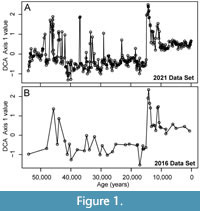To demonstrate the simulation framework and test the effect of different sampling protocols and environmental conditions on the recovery of paleoceanographic events, we use benthic foraminiferal assemblages that were previously analyzed to detect abrupt low-oxygen events in the Gulf of Alaska (GoA) over the last 54 ka as a case study (Figure 1; Sharon et al., 2021; Belanger et al., 2016). Integrated Ocean Drilling Program Site U1419 and the co-located jumbo piston core EW0840-85JC were cored on the continental slope at Khitrov Bank in the Gulf of Alaska at water depths of 697 m and 682 m, respectively (Jaeger et al., 2014). This places the site in the upper oxygen minimum zone where the modern oxygen concentration is ~0.59 ml/L (Paulmier and Ruiz-Pino, 2009; Garcia et al., 2013). Previous studies found that the first axis from a DCA analysis of these assemblages summarized variation in the relative abundance of species known to be dominant in low-oxygen settings. For example, Buliminella tenuata, Bolivina seminuda and Takayanagia delicata are all associated with dysoxic settings and have high positive DCA-1 scores whereas species associated with oxic settings, such as Pyrgo spp. and Quinqueloculina spp. had negative DCA-1 scores (Sharon et al., 2021). Geochemical proxies for oxygenation corroborated the oxygenation gradient along DCA-1 and samples with high DCA-1 scores also had high concentrations of redox sensitive metals such as Mo and U (Sharon et al., 2021). Thus, DCA-1 could be used to quantify the magnitude of changes in oxygenation and recovered dysoxic events (oxygenation < 0.5 ml/L O2) during the early Holocene, Bølling-Allerød, and MIS 3 (Sharon et al., 2021). These events ranged from ~4,000 years to <300 years in duration and changes in oxygenation frequently exceeded 1 ml/L O2 per 100 years, as evinced by rapid increases in the relative abundance of B. tenuata, B. seminuda and T. delicata from <10% of the assemblages during background conditions to as much as 80% of the assemblages during these events. The presence of laminations indicates that bioturbation by metazoans was limited during the low-oxygen portions of the record (Jaeger et al., 2014; Penkrot et al., 2018).

Simulating Fossil Assemblages along Environmental Gradients

In order to create a gradient of faunal assemblages from which to draw simulated assemblages, we modeled the original faunal counts along an ordination axis as smoothed distributions using kernel density estimates (KDEs) for each species. The original counts had a median of 268 individuals per sample (interquartile range = 159-404) and analyses relied on 48 taxa, which excluded 26 taxa that either occurred in only one sample or comprised fewer than 2% of individuals in all samples where it occurred (Sharon et al., 2021).

In fitting kernel densities to our data, we assume that species abundances have a non-monotonic, asymmetrical distribution with respect to the primary environmental gradient, defined here as the first score of a detrended correspondence analysis (henceforth, “DCA-1 value”), consistent with previous modeling of ecological gradients (Holland, 1995; Holland and Patzkowsky, 1999; Patzkowsky and Holland, 2012). To estimate species abundance along DCA-1 independent of the number of specimens, we calculate the proportional abundance of each species in each sample (shown in Figure 2A) and multiply that value by 10000. By multiplying the proportional abundance by 10000, we obtain the expected abundances of each species assuming a sample size of 10000 specimens; this is an order of magnitude larger than the sample size of any given sample in our case study data set and thus permits smoothing of the data before fitting the kernel density estimate. To ensure the model is not affected by the number of samples that were collected at a particular DCA-1 value in the original data set, we then average these abundances across those samples which each species was sampled from, within 20 equal sized ranges of DCA-1 values (Figure 2B). This provides the expected abundance of each species along DCA-1 as if a sample of 10000 individuals were obtained from each of the 20 segments (Figure 2C), conditioned on actually sampling the species at all. DCA is performed using the decorana function in the R package vegan (Oksanen, et al., 2022). Separate kernel density estimators are fit to each of these expected abundance distributions using the function density in the R package stats (R Core Team, 2022). This provides a kernel function describing the rise and fall of each species along DCA-1 with an arbitrary absolute height derived from the kernel density estimate (Figure 2D). We convert the KDE back to abundance estimates by scaling each species distribution such that the minimum and maximum heights of the KDE function match the minimum and maximum mean proportional abundance, as measured for each of the 20 bins.

The kernel density estimates for each species abundance is conditioned on the species being sampled at all, which necessitates that we first account for the probability that each species will occur in a sample. If a given species is present in all samples within a DCA-1 range previously used to derive the KDE, then the species has an occurrence probability of 100% within that range of DCA-1 values. However, if the species only occurs in one of 10 samples in a given DCA-1 range the species has an occurrence probability of 10%. To stochastically test whether a species indeed occurred in an assemblage being simulated at a given DCA-1 value, the algorithm randomly draws a number between zero and one for every species in the empirical data set and compares that number to the probability of occurrence for each species at that specific DCA-1 value. If the value drawn by the algorithm is greater than the probability, we calculated from the DCA range inclusive of the focal DCA-1 value, that species will have a non-zero probability of occurring in the assemblage.

Now that the algorithm has determined which species could occur within a simulated assemblage, we can calculate the expected relative abundance of each species by obtaining the value of the rescaled kernel density function of each species at that specific DCA1 value (i.e., a point somewhere on the horizontal axis of Figure 2D). Species that were not sampled by comparing the randomly drawn values to the probabilities of occurrence have these kernel density values set to zero. We treat the resulting values as weights which are relative to the expected proportional abundance of each species. We divide these kernel-derived weights by their sum, added up across all species, such that values for all species add to one. We treat these final values as the expected proportional abundance of each species in our simulated assemblage. To randomly draw specimen counts to generate an assemblage with a finite number of specimens in the model, we randomly sample a number of times (i.e., a number of individuals) with replacement, where the proportional probability of drawing each species is the expected proportional abundance.

To determine if paleoAM generates assemblages that are similar to the original fossil assemblages, we performed a series of simulations at the empirical DCA-1 values from the original GoA study. We simulated sets of 300 assemblages generated at the same DCA-1 value and number of individuals as each original fossil assemblage (see Appendix 1 for simulated abundance distributions). If our simulations produce assemblages similar to the fossil data set, there should be high fidelity between the simulated assemblages and the fossil assemblages in terms of species richness, evenness, pairwise dissimilarities, and recovered DCA-1 values. We measure evenness as Hurlbert’s probability of interspecific encounter (PIE), which is a commonly used metric of evenness of biodiversity (Hurlburt, 1971). PIE values are bounded at zero and one with zero indicating assemblages that are dominated by a single taxon and one representing assemblages in which all taxa are equally represented. Pairwise dissimilarities are calculated using the Bray-Curtis metric in the vegdist function of the R package vegan (Oksanen, et al., 2022). To overcome the sensitivity of DCA to changes in the underlying data (Kenkel and Orloci, 1986; Wartenberg et al.,1987; Jackson and Somers, 1991), we ordinated each simulated sample with the original fossil assemblages from the 54 ka GoA record. This approach allows the empirical data to dominate the structure of the ordination space and maintain the same structure between analyses that place individual simulated assemblages within that space. With both the simulated assemblages and the original fossil assemblages in the same ordination space, and thus on the same quantitative scale, we can calculate the difference between the DCA-1 value of the original fossil assemblage and the median DCA-1 value of the associated simulated assemblage set. To ensure any differences between the simulated and original assemblages were not simply due to a change in the ordination space, we also compared the median DCA-1 values of simulated assemblages to the median DCA-1 value of the original assemblage as recovered from the analysis.

We developed paleoAM in R version 4.2.0 (“Vigorous Calisthenics”) released on April 22nd, 2022, which uses an open-source programming language (R Core Team, 2022). All code needed to simulate fossil assemblages along an environmental gradient and perform the experiments described below are available as supplementary materials (Appendix 2).

Simulating the Deposition of the Fossil Assemblages

To test whether changes in faunal composition can be detected within a time series, we simulated a stratigraphic record of faunal assemblages with a given background DCA-1 value that is punctuated by assemblages with higher DCA-1 values (“events”; Figure 2E). The resulting sequence of assemblages can be conceptualized as a series of discrete “assemblage packages,” which are accumulations of specimens deposited in 1 year within the model under the environmental conditions implied by the generating DCA-1 values. Events are separated by relatively long periods of background conditions in the simulated record and the event waiting periods have randomly varied errors added to their duration, thus randomizing when individual events occur in each record.

We then sample each simulated sedimentary record within defined intervals, hereafter the “sample interval,” which is conceptually like obtaining a sediment sample with a prescribed thickness from a continuous sediment core. Given the record is sampled at equally spaced intervals and events occur randomly, sample intervals vary stochastically in the relative number of assemblage packages that they incorporate from background and event conditions. However, the long waiting periods between events ensure that no sample interval intersects more than one event. To create a sample, we draw 400 specimens from each assemblage package intersected by the sample interval and amalgamate them into a “meta-assemblage,” which effectively time-averages the sample. We then subsample the meta-assemblage to obtain the 300 specimens that constitute the recovered faunal sample corresponding to the sample interval. We use 300 specimens as the sample size following the recommendation of Buzas (1990), however, smaller sample sizes often produce stable ordination results (Forcino et al., 2015); this is comparable to the median 268 individuals per sample in Sharon et al. (2021).

In simulating the sedimentary records by sequentially accumulating discrete assemblage packages that each have a microfossil assemblage reflecting the community composition at a defined position along an environmental gradient, we establish an initial, ideal record. We can then explore the effect of varying the duration of the events the magnitude of environmental change during events and the duration of the transition between background and event intervals by changing the model parameters used to create the record (Table 1). In addition, we can test the effect of the relative completeness of sampling by varying the distance between sample intervals. Further, we can simulate the effects of mixing via bioturbation by altering this initial simulated sedimentary record.

We define event detection as the ability to differentiate a sample from the background environmental conditions and detection accuracy as the similarity of the sample to the generating DCA-1 value. To produce a null distribution against which to test a DCA-1 value, we simulate 100 assemblages at the background DCA-1 value and 100 assemblages as the event DCA-1 value. We then calculate the upper 95% quantile of the DCA-1 values of assemblages simulated at background conditions and calculate the two-tailed 95% quantile of the DCA-1 values of assemblages simulated at event conditions. Samples that return DCA-1 values outside the 95% quantile of the simulated background are considered significantly outside the expected noise in DCA-1 values for assemblages at the background value, and thus signifies a “detected” event. We consider an event to be “accurately detected” if a sample also has a DCA-1 value within the 95% quantile of assemblages simulated at the event conditions. To consider the different contributions of event detection and the accurate recovery of DCA-1 values on accurate detection, we calculate the median excursion magnitude across all samples that intersect an event in the simulation; in contrast, accurate detection only requires one qualifying sample per event. Note that different events within a simulation may be intersected by different numbers of samples, and samples can have variable contributions from event assemblages and background assemblages. We use the surface of median excursion magnitudes calculated across simulations at different combinations of model parameters to illustrate the general trend of recovered DCA-1 values as excursion magnitudes and resolution potential increases.

Varying resolution potential of the sedimentary record. We simulate events with a fixed temporal duration, however, differences in sediment accumulation rate will affect the thickness of the sedimentary interval over which the event is recorded and, thus, the potential for capturing the event within a sample interval of defined thickness. To incorporate this behavior, our simulations are executed on a ratio reflecting the resolution potential of event sampling, which encompasses the event duration, sediment accumulation rate and thickness of the sample interval. Resolution potential describes how long an event is relative to the amount of time represented by the sample interval and is calculated as the product of the duration of events (in units of time) and the sedimentation rate (in units of depth added per unit of time, e.g., centimeters per year), divided by the thickness of the sample interval (in units of core depth, e.g., centimeters). Thus, in a record with a resolution potential of one, a sample is as thick as the amount of sediment laid down during the event’s duration. For example, for a typical deep-sea marine sediment core with a sedimentation rate of 0.01 cm/yr over a thousand-year timespan (Sadler, 1999), a resolution potential of one would result if samples were 1 cm thick and the target event is 100 years long. In marine sedimentary records, sedimentary intervals of 1 to 3 cm thick are commonly needed to achieve sufficient foraminiferal abundances for statistical analyses. The larger samples are often necessary to obtain these abundances in high sedimentation rate records due to sedimentary dilution of the fossil material. However, the effect of sample thickness on resolution potential may be balanced by an expanded sedimentary interval representing a given time span. For example, on continental shelves where typical sedimentation rates are 0.5 cm/yr when measured on thousand-year timespans (Sadler, 1999), even a 3 cm thick sample would result in a resolution potential of 16.7 for 100-year events, although the resolution potential would be only 1.67 for 10-year events. Other studies observed that climate events of shorter duration are more severely attenuated (Anderson, 2001; Steiner et al., 2016; Liu et al., 2021), which is reflected here in the lower resolution potential of shorter events. For each time series scenario simulated herein, we vary the resolution potential to test how the amount of time represented by the sample interval relative to the duration of the event affects our ability to detect the event and accurately estimate its magnitude. We vary resolution potential in the time-series simulations across three orders of magnitude with values every 0.05 units from 0.05 to 0.2, then every 0.1 units from 0.2 to 0.5, then every 0.5 units from 0.5 to 7 units.

Varying the magnitude of the excursion. We expect the difference between background and event conditions to have a large effect on our ability to detect events. Although DCA Axis 1 is scaled with respect to the standard deviation of faunal variation, differences in the species composition and the relative abundance structure at different positions on the gradient could affect the distinctiveness of background and event assemblages. Thus, to test the effect of magnitude of the excursion on detecting events and accurately estimating the degree of faunal change, we vary both the background DCA-1 value and the event DCA-1 value (Table 1). The difference between these two values is termed the “excursion magnitude.” We use background values of -0.5, 0.5 and 1.0 and maximum excursion magnitudes which range up to 2.996, 1.996 and 1.496, respectively, which are constrained by the maximum DCA-1 value (2.496) obtained from ordinating the original fossil assemblages. Simulations were run with excursion magnitudes in 0.2-unit increments between zero and the respective maximum excursion magnitude for that simulation.

Testing the Effects of Transition Duration, Sampling Completeness and Bioturbation

The change from background to event conditions may occur nearly instantaneously or occur gradually over a transition interval. To test the effect of the abruptness of events on their detection, we varied the duration of the transitions between background and event conditions. Each event interval is both preceded and followed by a transition interval, during which the DCA-1 value transitions linearly from the background value to the event value, or vice versa. The duration of the transitions is parameterized in our model as a multiple of the event duration. Values much less than one give transition intervals that are very small with respect to event durations and, thus, simulate extremely abrupt transitions. When the transition is abrupt, the resulting meta-assemblages are composed of very few assemblages with transitional DCA-1 values, thus the meta-assemblage is primarily composed of assemblages generated under either the event DCA-1 value, the background DCA-1 value or a mixture of both. Transition durations longer than the event duration maximize the probability that samples will intersect intervals simulated at intermediate DCA-1 values within the transition interval.

Sampling completeness, here defined as the proportion of the sedimentary core record that is contained within the sample intervals, can also affect the detection of events from a sedimentary record. We do not consider the loss of individuals to taphonomic processes in our analyses of completeness. Thus, we consider sampling to be 100% complete if all potential sample intervals across the entire sedimentary core are sampled. We parameterize sampling completeness as a value between zero and one, where one is a completely sampled core in which each observed sample is immediately adjacent to the following sample. Sampling completeness values less than one result in intervals of unsampled sediment between recovered samples. Sedimentary records are rarely completely sampled and, on average, a record in which only 25% of the record is sampled for fossils (e.g., a sampling completeness of 0.25) will miss three out of every four events assuming the events are shorter than the sample spacing. For most simulations, we use a sampling completeness of one, which equates to sampling the total sedimentary core record. To test the effect of sampling completeness on event detection, we compare this scenario of complete sampling to a scenario in which we only observe every fourth potential sample in the time series, skipping a stratigraphic interval equivalent to three samples between each sample (sampling completeness = 0.25).

The movement of sediment by burrowing or feeding organisms (bioturbation) and other sediment movement cause particles of sediment, including fossils, deposited at a particular point in time to mix with particles deposited at a different time. Bioturbation is known to homogenize sediments deposited under different environmental conditions and can limit our ability to reconstruct abrupt events from fossil assemblages (Berger and Heath, 1968; Martin 1999). In paleoAM, we model bioturbation as the inclusion of specimens from assemblage packages above and below the designated sample interval in the simulated sedimentary record. Thus, bioturbation is a process in which a sample is infiltrated by specimens from assemblage packages adjacent to the designated sample interval. Although bioturbation can also displace specimens, and thus the signal of an event, downward in the sediment column (Berger and Heath, 1968), paleoAM does not detect an event if it is displaced outside of the assigned event interval.

In the simulations, the intensity of bioturbation can vary from zero to one. Zero bioturbation intensity implies that all specimens are drawn from assemblage packages within the designated sample interval. All simulations in this paper conducted “without bioturbation” were conducted at a bioturbation intensity of zero. When bioturbation intensity is equal to one, specimens contained in the final sampled assemblage will be drawn from both assemblage packages within the designated sample interval as well as from adjacent packages. This results in complete mixing of the microfossil assemblages across the bioturbation interval. Although we do not simulate intermediate bioturbation intensities in this study, focusing instead on the end-member values of zero and one, this parameter can be adjusted in paleoAM. For example, if bioturbation is set to 0.5, the proportion of specimens mixed into the final assemblage from assemblages outside of the sample interval will be halved (and the proportion of specimens from the designated sample interval itself will be doubled).

In all simulations where bioturbation occurs, we treat the thickness of the bioturbation interval as a function of the thickness of the sample interval, fixed to a ratio of 10 over three. This is based on the typical 3 cm sample thickness in the GoA data set examined and the typical 10 cm depth of bioturbation in modern marine sediments (Boudreau, 1998; Teal et al., 2008; Teal et al., 2010; Tarhan et al., 2015). Effectively, the zone of bioturbation is always 3.3 times larger than the sample interval regardless of the resolution potential. Although others allow bioturbation to attenuate in intensity with depth, vary over time with environmental change or operate asymmetrically in their models (Trauth 1998; Bently et al. 2006; Löwemark et al., 2008; Trauth 2013; Hülse et al., 2022), we keep bioturbation constant and its effect symmetrical across these 10 cm. This degree of bioturbation is likely an overestimate for this record because the GoA data set was at least partly deposited under suboxic to dysoxic conditions and contains well-preserved laminations indicating a lack of bioturbation in some intervals (Jaeger et al., 2014; Belanger et al., 2016; Penkrot et al., 2018; Sharon et al., 2021). The depth of bioturbation typically decreases as oxygenation decreases (Teal et al., 2008; Solan et al., 2019) and Smith et al. (2000) reported that the depth of the bioturbated mixed layer is ~5 cm thick in dysoxic regions (0.13-0.27 mL/L bottom-water oxygen). Further, a fixed interval of bioturbation ignores the eventual sediment compaction of the core such that simulated bioturbation occurs over the modern, shortened core, rather than over the more expanded sedimentary interval at the time of deposition (Jaeger et al., 2014; Walczak et al., 2015). However, given the importance of bioturbation found by previous studies (i.e., Anderson, 2001; Steiner et al, 2016; Liu et al., 2021), we prefer to bias these analyses toward overestimating the effects of bioturbation rather than mistakenly diminishing its effect.

Simulations of Mixed Assemblages

The true magnitude of change during an event might be underestimated when samples contain mixtures of fossils that accumulated at different times, either because bioturbation has homogenized the sample interval or because the sample interval straddles sediments deposited under different environmental conditions. Thus, an investigator using a faunal assemblage proxy may want to reconstruct the range of possible true event values that could be represented by the empirical DCA-1 value they observe. To directly examine the relationship between the true event values and observed DCA-1 values, we use a set of simpler models that isolate the effects of event value and the proportion of the sample that comes from the event interval. Each assemblage in this simulation is a mixture of two end-member assemblages that were generated at a background value (-0.5 DCA-1 units) and across different true event values. This abstraction avoids the confounding effects of our more complex time-series simulations and allows us to estimate how the frequency of a particular empirical DCA-1 value varies with the event value and the degree of mixing between the event and background assemblages. For these simulations, we generated 100 samples of 30000 individuals at 101 prescribed mixtures of assemblages simulated at background and event values. The relative contribution of specimens from event intervals and background intervals to sampled assemblages ranged from 0 to 100% of background in increments of 1%. The resulting meta-assemblages are sub-sampled to 300 individuals to obtain the final sample of observed specimens. We examined the distribution of DCA-1 values produced by each set of 100 samples to determine the frequency at which combinations of true event values and proportional contributions of the event assemblage would produce the observed DCA-1 values.

Making a Sampling Plan from Pilot Samples

We further demonstrate how an investigator might use the paleoAM framework with a set of pilot samples to estimate the sampling frequency and sample thickness necessary to reliably resolve short-lived environmental perturbations and make an informed sampling plan. To simulate a limited set of pilot data, we combined faunal data from 29 samples from Site U1419 (Belanger et al. 2016) and 18 samples from the co-located site survey core (EW0408-85JC) collected in 2008. These samples span the full 54 ka record at lower resolution than the dataset published in Sharon et al. (2021) and represent what an investigator would have had as a pilot data set in 2016 while planning a higher resolution study (Figure 1). We test whether an investigator using paleoAM with this smaller 47 sample data set would come to similar conclusions about the type and frequency of sampling necessary as an investigator working from the larger 355-sample record from 2021. For this scenario, we assume the investigator is interested in testing whether low-oxygen events similar in duration to those recorded elsewhere in the North Pacific occur at the study site. Previous studies in the Santa Barbara Basin (Cannarito et al., 1999, Ohkushi et al., 2013) suggest some late Pleistocene dysoxic events are as brief as a few decades or longer than a millennium. Thus, we estimate the probability of capturing events of different magnitudes that are 50, 100 and 1000 years in duration, with incomplete sampling (25% completeness), abrupt transitions (0.001 times the event length) between event and background (DCA-1 value = -0.5) and under scenarios with and without bioturbation. We also vary the sample thickness at 1, 2 and 3 cm because the investigator can often choose the sample thickness and volume they acquire when sampling a core.

Assessment of Event Detection in an Existing Record

We further performed post-hoc exploratory simulations to assess the ability of the record to detect events of specified durations after the investigators have completed sampling and counting of their fossil data set. In the GoA record (and in almost any sedimentary archive), rates of sedimentation vary over the record and, thus, an even sampling plan based on core depths will not result in a consistent resolution potential throughout the record. We can calculate a time-varying resolution potential for a record for a given event duration we wish to resolve, based on the sample thickness used and estimates of the time-varying sedimentation rate. Published sedimentation rates for this record, which were calculated as the median rate in 500-year intervals based on radiocarbon data using the Marine20 calibration, average ~200 cm/ka during the glacial portion of the record (older than ~18 ka) and are as high as 800 cm/ka during the deglacial interval, but decrease to an average of 50 cm/ka during the last 12 ka Walczak et al. (2020). These are exceptionally high sedimentation rates related to the site’s position on the continental slope near a source of glacial erosion (Jaeger et al., 2014; Walczak et al., 2020). We use this time series of sedimentation rates in the original 500-year intervals to determine the time-varying resolution potential of the record for events with a 100-year duration. These estimates of resolution potential assume a 3 cm sample thickness, although true sample thickness varied, with some samples being 2 cm thick (Sharon et al., 2021). We choose to use 3 cm thick samples in the simulation, as this represents a worst-case scenario, and should underestimate our ability to resolve events of 100-year duration. We then use this time-series of resolution potentials to simulate the probability of detecting 100-year events along the record and determine the magnitude of events that would be recorded by resulting assemblages if an excursion magnitude of 0.4, 1.2, and 2.8 DCA-1 units occurred. Given this context, we examine the original record to assess whether events were likely to be unsampled in the high-resolution record or were likely to be recovered at a lower apparent DCA-1 value than the true event value.

RESULTS AND DISCUSSION

Validating the Simulation Model

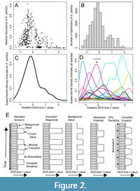
Since DCA was devised by Hill and Gauch (1980), there has been an active debate about the arbitrary aspects of its algorithm and the theoretical potential for introducing distortion into the resulting ordination (Kenkel and Orloci 1986; Faith et al., 1987; Minchin, 1987; Wartenberg et al., 1987; Peet et al., 1988; Jackson and Somers, 1991; Oksanen and Minchin, 1997; Faith, 1999; Olszewski and Erwin, 2009; Patzkowsky and Holland, 2012). Thus, concern about the ability of DCA to reproducibly place simulated assemblages across the entire gradient may arise. Further, DCA could place simulated assemblages in the correct order along the gradient but fail to capture the DCA-1 values themselves, obscuring the use of DCA-1 values in generating a quantitative oxygenation proxy. Given we only provide the simulations with information about species distribution along DCA-1, simulated assemblages produce the full range of DCA-1 values but produce a limited range of values along DCA-2 (Figure 3A). For each simulated assemblage, the recovered DCA-1 value is close to the generating DCA-1 values from simulation (Figure 3B). The median DCA-1 value of each set of 100 simulated faunal assemblages closely replicates the target DCA axis 1 value with a mean difference of 0.01 DCA units (two-sided 95% quantiles: -0.021 to +0.057 units). Similarly, the median recovered DCA-1 values of the original fossil assemblage were well replicated by the new DCA space with a mean difference of 0.01 DCA units (95% quantiles: -0.022 to +0.06). The range of DCA-1 values in the original data set is -1.309 to 2.496, thus this difference is <1% of the range in DCA-1 values in both cases. Thus, we are confident that the DCA-1 gradients we simulate are reproducible and reasonably reflect that ecological gradient, but other DCA axes are not reliable.

While our simulated assemblages recovered the generating DCA-1 values well, they less precisely replicate standard ecological metrics, such as taxonomic richness and evenness, and the overall pairwise compositional dissimilarity among assemblages. Taxonomic richness in the empirical dataset varied from five to 33 taxa per sample whereas the median richness of the simulated assemblage sets is, on average, 1.37 species greater (two-sided 95% quantiles: -6 to +6 species) than the richness of the empirical sample with the same DCA-1 value. The median PIE from simulations is also greater than the empirical sample by a mean increase of 0.077 units (95% quantiles: -0.059 to +0.34); in the empirical dataset, the samples have PIE values from 0.32 to 0.96. The Bray-Curtis dissimilarity among pairs of simulated assemblages is often lower than the dissimilarity among empirical assemblage pairs, although very high dissimilarities and dissimilarities between 0.5 and 0.75 are more reliably replicated (Figure 3C). In simulating the assemblages, paleoAM models abundance distributions along DCA-1 only and ignores all other faunal variation present in the empirical samples, which drives the greater similarity. Richness and evenness may be higher in the simulated assemblages because we are sampling from continuous abundance distributions whereas species in natural benthic communities often occur in disjunct patches, reflecting the influence of environmental factors on organism distributions that are not captured on the single axis of faunal variation we analyze here (Ardisson and Bourget, 1992; Fabri-Ruiz et al., 2019). The assumption that species distributions are continuous and unaffected by factors whose influence may be captured on additional axes of faunal variation will enhance richness and evenness at all points of the gradient because it causes rare taxa that infrequently occur in natural communities to be sampled more often (Appendix 1). Taken together, these metrics show that the simulations do not capture the full faunal variation present in the empirical dataset even though they replicate DCA-1 well.

Effects of Excursion Magnitude and Resolution Potential on Event Reconstruction

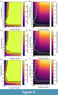We simulated events against three different background levels with DCA-1 values of -0.5, 0.5 and 1. To compare results across simulations, we normalize the event DCA-1 values relative to the background using the excursion magnitude, which is calculated as the difference between background and event DCA-1 values. Therefore, a simulation may have the same excursion magnitude but have very different event and background assemblages drawn from different portions of the DCA-1 gradient. In Figure 4, we depict the percentage of events that are accurately detected (left panels) and the median recovered excursion magnitudes (right panels) for all simulated combinations of excursion magnitude and resolution potential. Each row of panels in Figure 4 is simulated at a different background value, however, the results are similar for similar excursion magnitude - resolution potential pairs. For example, median recovered excursion magnitudes are depressed relative to the generating excursion magnitude at resolution potentials less than 3 units, but are equivalent, on average, to the generating excursion magnitude at resolution potentials above 3 units. This means that events have a similar probability of being accurately detected at similar combinations of excursion magnitudes (the deviation from the background DCA value during the event) and resolution potentials (the ratio of sample thickness to event duration). This consistency indicates that the portion of DCA-1 gradient over which we simulate change has a minimal impact on our results. Thus, we will focus our discussion on those simulations with the minimum background DCA-1 value of -0.5 (as in Figure 4A and 4B).

In simulations where events are abrupt, bioturbation is absent, and sampling is complete, more than 95% of events are accurately recovered when resolution potential is >2 units and excursion magnitudes are greater than 0.2 DCA-1 units (Figure 4). As excursion magnitude increases, the resolution potential necessary to accurately detect 95% of events decreases until excursion magnitudes reach ~0.6 DCA-1 units after which the resolution potential needed to accurately resolve events increases. Excursion magnitude has a minimal effect on event reconstruction when resolution potential is greater than 1.2 units as indicated by the near vertical probability contours in Figure 4. At resolution potentials <1 unit, events are accurately detected in less than 50% of simulations.

The inflection of the accurate detection contours at excursion magnitudes of -0.6 DCA units (Figure 4) is driven by the interaction between event detection and detection accuracy. When event values are simulated close to the background value (simulations with low excursion magnitudes), the event values recovered from the simulation are very close to the generating values of the event, and thus have high accuracy, but they are not far enough from the background value to be distinguishable as an event. Events that are very different from the background (simulations with high excursion magnitudes) will be easy to differentiate from the background, and thus are easily counted as “detectable” events, but they are much more likely to be inaccurately recovered, which is seen in the lower median recovered excursion magnitudes where the generating excursion magnitudes are high and resolution potential is less than 3 units (Figure 4B). Thus, when an event is detected, it is likely that the event is attenuated in amplitude and could represent a true event of higher magnitude. At intermediate event values, the event is far enough from the background value to be detected and the attenuation of the event value in the recovered sampled is minimal because individuals from background assemblages are like those in event assemblages and, thus, intermediate event values are the most likely to be accurately detected.

Effects of Transition Duration, Sampling Completeness and Bioturbation on Event Detection

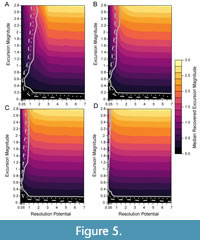With longer transitions between background and event intervals, the ability to accurately detect events increases even for events simulated in low-resolution potential records (Figure 5). As the duration of the transition increases from nearly instantaneous (Figure 5A) to five times greater than the event interval (Figure 5D), the ability to accurately detect events in simulations with lower resolution potentials gradually increases because the recovered excursion magnitudes are, on average, higher. This higher median excursion magnitude occurs because the transition interval contains assemblages generated from DCA-1 values that depart from background and more individuals from event-like assemblages are incorporated into the sample, increasing the recovered DCA-1 value. Thus, events that are effectively lengthened by transitional intervals will be easier to detect in sedimentary records even though transitional assemblages have lower DCA-1 values than the event itself.

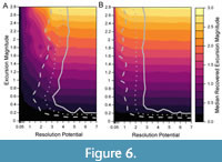When sampling completeness is reduced to 25%, a resolution potential of 3–4 units is necessary to detect events in 95% of simulations (Figure 6), higher than the resolution potential of 0.5–2 units needed for events with the same transition durations when sampling is complete (Figure 5A, 5D). Although the proportion of events that are accurately detected are lower in the incomplete records, the median recovered excursion magnitudes remain like the simulations performed at 100% completeness (Figure 5, Figure 6). This demonstrates that the reduction in the percentage of accurately detected events is purely because the events are unsampled. Thus, incomplete sampling will reduce the probability that an event is detected but will not affect the perceived magnitude of the events that are detected.

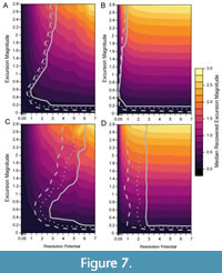When bioturbation is included in simulations (Figure 7), the percentage of events that are accurately detected decreases at low resolution potentials compared to simulations without bioturbation, as shown in Figure 8, which depicts the percentage of events accurately detected in simulations without bioturbation subtracted from the percentage of events accurately detected in simulations where bioturbation occurs (Figure 5, Figure 6). Despite this decrease in accurate detection with bioturbation at low resolution potentials, >95% of events are still accurately detected in the presence of bioturbation when resolution potential is >3, sampling is complete, and transitions are short (Figure 7A). Although accurate detection is similar with and without bioturbation for completely sampled records (Figure 8A, 8B), bioturbation enhances the decrease in median excursion magnitudes recovered at decreasing resolution potentials when the transition duration is short (Figure 7A). In contrast, bioturbation has little effect on the median recovered excursion magnitude when the transition duration is five times the event duration (Figure 7B). These simulations ignore apparent excursions that occur in samples that do not intersect the event interval. However, given bioturbation would also mix individuals from event assemblages into adjacent assemblage packages deposited under background conditions, an event could be detected outside of the event interval in practice. This would cause an event to be temporally offset, as seen in other simulations (Hulse et al., 2022). If multiple samples were to intersect a bioturbated interval containing an event, the event could also appear longer in duration when recovered as a time series.

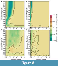Reducing sampling completeness to 25% primarily affects the resolution potential necessary to accurately detect events. Whereas >95% of events with short transition durations (0.001 times the event duration) are accurately detected in completely sampled records when resolution potential is >3, resolution potentials must exceed 6 units when sampling is reduced to 25% and bioturbation occurs (Figure 7C); the necessary resolution potential is lower in the absence of bioturbation (Figure 6A, Figure 8C). Similarly, although >95% of events with long transition durations (5 times the event duration) are accurately detected in completely sampled records when resolution potentials are >1, resolution potentials must be >3 to accurately detect high magnitude excursions at 25% completeness both with and without bioturbation (Figure 6B, Figure 7D, Figure 8D). Despite differences in accurate detection, the median excursion magnitudes recovered are very similar between simulations at different completeness holding transition duration constant (Figure 5, Figure 6, Figure 7).

The worst-case scenario that we consider simulates events with short transition durations, incomplete sampling, and bioturbation (Figure 7C, Figure 8C). In this scenario, abrupt events are both attenuated by bioturbation (as in Figure 7A, Figure 8A) and missed due to not being sampled (as in Figure 6A). The combined effect of these parameters reduces the probability of detecting events with high excursion magnitudes such that recovering larger excursions requires increasingly higher resolution potentials. When these high magnitude events are detected, they will be most likely detected as lower magnitude excursions, making it difficult to differentiate between events of different magnitudes in incompletely sampled, bioturbated, sedimentary records, particularly at low resolution potentials.

Other studies also find that bioturbation decreases the amplitude of events and that abrupt events are best preserved when sedimentation rates are high and bioturbation low (Anderson, 2001; Steiner et al, 2016; Liu et al., 2021), however, the impact of bioturbation is greater than what our simulations imply. For example, the amplitude of 4 ka long events decreased by 50% at a sedimentation rate of 10 cm/ka and by 20% at a sedimentation rate of 20 cm/ka (Anderson, 2001). If records with these sedimentation rates were sampled with 3 cm samples, as done in our case study, this would equate to resolution potentials of 13.3 and 26.6 units, respectively, for 4 ka events. Thus, the attenuation forecast by the model in (Anderson, 2001) has a much greater effect than we estimate in our simulations, where the vast majority of events are accurately detected at much lower resolution potentials. In the simulations in Anderson (2001), sedimentation rates had to exceed 70 cm/ka for the attenuation of the record to decrease below 5% for events with a period of 2 ka (with 3 cm thick samples, this would be an equivalent resolution potential of 46.6 units). Similarly, other simulations demonstrated that centennial-scale climate variability could not be preserved when bioturbation occurred over a 10 cm depth even when sedimentation rates exceeded 15 cm/ka (Liu et al., 2021). However, these earlier studies focused on geochemical records (i.e., δ¹⁸ O derived from multiple foraminiferal tests) and our differing results could suggest that environmental proxies derived from multi-taxon faunal assemblages are less sensitive to mixing. Further, the simulations herein treat assemblages as accumulations of independently mobile particles from which the proxy value is derived whereas the approaches in Anderson (2001) and Liu et al. (2021) impose the effect of time-averaging and bioturbation on isotopic signals using mathematical convolution, with the change in the isotopic curve based on the mixing effect observed in empirical studies (respectively, Ruddiman et al., 1980, and Guinasso and Schink, 1975). Other simulations focused on geochemical data derived from foraminifera do simulate foraminifera as particles but modeled assemblages of at most two species (Trauth, 1998; Löwemark et al., 2008; Trauth, 2013; Hülse et al., 2022). Although we treat the foraminifera tests as independent particles, we do not consider size selective mixing, which could impact the resulting faunal assemblages as well as the isotopic records derived from those tests (Hupp et al., 2019). Potentially confounding dissimilarities in model mechanics and underlying proxies make it difficult to discern the cause for our contrasting conclusions about the impact of bioturbation on accurately detecting climate events and future work systematically comparing the models on the same datasets would be informative.

Simulations of Mixed Assemblages

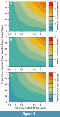If an investigator observes a given DCA-1 value from an empirical sample, that value may have resulted from a multitude of possible combinations of event values and relative contributions of the event assemblage to the observed sample. Empirical samples will contain individuals from outside the event assemblage whenever (a) the event duration is longer than the time represented by the sample interval, (b) the entire sample is not contained within the event interval, or (c) bioturbation has mixed in individuals from background assemblages. The proportional contribution of the event assemblage to the empirical sample may also be affected by the differential production of individuals during different environmental conditions and through the differential taphonomic disintegration of taxa (Tomašových et al., 2019), and thus, also affect the reconstruction of events. Simple simulated mixtures of event assemblages and background assemblages demonstrate how the interaction between the true event value and the relative contribution of event assemblages to a sample produce different DCA-1 values (Figure 9), but do not currently accommodate differences in production and disintegration among taxa or assemblages. In general, empirical DCA-1 values will underestimate the true magnitude of events, given any contribution of the background assemblage to the observed sample will bias the observed DCA-1 value towards the background DCA-1 value. Thus, it would be uncommon to observe high DCA-1 values in an empirical sample even if an event with a high DCA-1 value occurred, unless there was little to no contribution from the background assemblage (Figure 9).

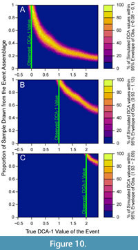These simulations also show that a given observed empirical DCA-1 value can only result from a relatively restricted combination of true event values and mixtures of event and background assemblages (Figure 10). In Figure 10, each panel depicts the proportion of simulations in which a given DCA-1 value is observed at all simulated combinations of true event values and relative contributions of the event assemblage to the observed sample. In each case, the empirical DCA-1 value matches the true event value when 100% of the sample is derived from the event assemblage, but that same empirical value is also observed when the true event value is higher, and the event contributes less than 100% of the sample; this is visualized as a narrow ridge of high probability in the plot space (Figure 10). Observed empirical DCA-1 values that are relatively high (Figure 10A, 10B), can only be produced when the event assemblage comprises most of the observed sample. Thus, if high DCA-1 values are observed, even if represented by only a single sample, they likely evince short-term, extreme, events and should not be regarded as noise.

These results also have implications for attempts to “unmix” faunal assemblages. When the observed DCA-1 value is high, the relationship with the resulting empirical DCA-1 values appears to decrease linearly as the proportion of individuals derived from event assemblages decreases. However, this relationship is nonlinear when we consider lower observed DCA-1 values (Figure 10A). Thus, unmixing routines for faunal proxies that assume that calculated assemblage metrics (such as ordination scores) change linearly with the amount of mixing may be inaccurate except for when very disparate assemblages are being mixed. In studies of time averaging, others have found that anomalous assemblages are noticeable even with high degrees of temporal mixing with background assemblages. For example, simulated mixing of terrestrial mammal faunas found that even when assemblages equally combine elements from two habitats the assemblages produced ordination results indicative of the more distinctive assemblage (Andrews, 2006). Further, time-averaged molluscan death assemblages preserved comparable pairwise dissimilarities as living assemblages from the same sites suggesting that fossil assemblages can retained much of their distinctiveness despite a dampening in average dissimilarity due to temporal mixing (Tomašových and Kidwell, 2009). Similarly, spatial heterogeneity among fossil assemblages is retained even when temporally mixed (Webber, 2005; Holland, 2005). In the case study herein, the dysoxic assemblage is distinct from the background assemblages both in taxonomic composition and in the high relative abundances of low-oxygen tolerant species (Sharon et al., 2021), which likely increases its recoverability. Further, the decline in bioturbation depth and intensity associated with oxygenation has also been shown to increase preservation of abrupt shifts in faunal composition on continental shelf (Tomašových et al. 2020) and plays a role in the recovery of low-oxygen events here as well. Previous studies of time averaging in macrofaunal shelly assemblages also suggest that even if assemblages overlap in time by 50%, the older assemblage will only contribute 10% of the fossils in the resulting sampled assemblage due to the exponential taphonomic loss of the fossils (Olszewski, 1999), thus the preserved assemblage mostly retains individuals of similar age. We do not include this loss of older specimens in the simulations herein, thus, the DCA-1 values we obtain from the simulations likely depart further from the event value than they would in a natural sedimentary system–unless the age frequency distribution of subsurface assemblages are more symmetric, as suggested by recent modeling work by Tomašových et al. (2023), and assemblage mixing would be greater than in Olszewski (1999), as in our model.

Using a Simulation Approach to Develop a Sampling Plan

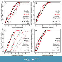Simulations based on the 2021 data set (355 samples) and simulations based on the 2016 data set (47 samples), have similar ability to accurately detect events, particularly when bioturbation is absent (Figure 11). When bioturbation is present, simulations based on the 2016 data are less able to accurately detect events of higher magnitude than simulations based on the 2021 data set, although detection itself is unaffected even when simulated with 25% completeness and short transition durations between background and event conditions. This indicates that a smaller dataset typical of a pilot study can be used in these simulations to inform further sampling and will achieve similar results as the high-density sampling of the 2021 data set. However, the selection of the pilot data was non-random in this case and was informed by lithological and geochemical environmental indicators such that the faunas reasonably spanned the full environmental gradient of interest even though samples were fewer. If the pilot data had spanned only a portion of the DCA-1 gradient, the similarity would not be achieved because the simulations cannot create assemblages outside of the sampled environmental gradient. The systematically lower detection accuracy when using the 2016 data set in bioturbated records could lead an investigator to oversample because a greater resolution potential is necessary to achieve a desired detection accuracy.

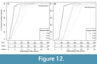Understanding the interaction between sedimentation rates, event duration and sample thickness, which we encapsulate in resolution potential, allows an investigator to modify their sampling design to maximize the detection of abrupt events. For example, an investigator has some control of sample thickness and thus could choose different sample increments depending on the number of fossil specimens expected in a volume of sediment (which is governed by sedimentation rates, preservation, and production of the target specimens). Given thinner samples contribute to higher resolution potential than thicker samples, the percentage of events that are accurately detected with 1 cm thick samples increases faster with increasing sedimentation rate than when sample thickness is 3 cm (Figure 12). The shape of the curves is the same regardless of event duration, however higher sedimentation rates are necessary to accurately detect events of shorter duration with a given sample thickness (Figure 12). The example is based upon excursion magnitudes of 2.8 DCA-1 units and simulations using the 2016 dataset, a scenario in which events are deliberately biased toward being less likely to be accurately detected (Figure 11). Given that accurate detection is more difficult for higher magnitude events (Figure 11), the percentage of events accurately detected would be higher for lower magnitude events. In this record, many of the samples were 3 cm thick and thus we would expect to accurately capture >95% of events that are 100 years long when sedimentation rates ~125 cm/ka even when sampling completeness is at 25%. Decreasing the sample thickness to 2 cm would allow 100-year-long events to be accurately detected provided sedimentation rates were at least 75 cm/ka, although sampling the time series with 2 cm thick samples would require more samples than at 3 cm to achieve 25% completeness. When sampled with 1 cm thick samples, millennial scale events (1000 yr duration) are detectable with >95% accuracy when sedimentation rates are at least 5 cm/ka and bioturbation is absent. Anderson (2001) found that comparable events were detectable at sedimentation rates as low as 5 cm/ka and undetectable at lower sedimentation rates, however, we find that some proportion of these shorter-term events would still be accurately detected even if allowing for bioturbation (Figure 12).

Assessment of Event Detection in an Existing Record

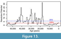These simulations also allow investigators to estimate the probability that (a) the events detected in a record are represented by assemblages that accurately reflect the environmental conditions and (b) the lack of observed events truly indicate the absence of events. Using simulations based on the 2021 record, we find that the resolution potential of the GoA record is sufficiently high to resolve >90% of 100-year events with DCA-1 values of 2.8 at 100% completeness (~73% of events at 25% completeness) prior to ~16 ka after which sedimentation rates decrease sharply (Figure 13). In some intervals, particularly since 16 ka, sedimentation rates were too low to accurately observe extreme 100-year events with 3 cm thick samples even when sampling is 100% complete, although the events are frequently detected as lower magnitude events than originally simulated (Figure 14). Less extreme events are more accurately detected, even when sedimentation rates are lower, indicating that low-magnitude events are more likely to be accurately recovered than the most extreme events (Figure 14). 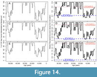Although we performed these simulations with bioturbation, intervals of the GoA record contained laminations suggesting minimal bioturbation (Jaeger et al., 2014; Penkrot et al., 2018), thus accurate detection of events may be greater than we estimate here. In a record with lower sedimentation rates where event detection would be more challenging, these simulations would permit an investigator to quantitatively support that the absence of an expected event of a given duration was due to low resolution potential and test whether the low resolution potential was the result of the sedimentation rates or the sampling strategy. These effects of sedimentation rates and sampling strategies on event detection need to be accounted for when comparing across multiple core records because an event may appear more extreme in one record than another simply due to differences in the resolution potential and not because that locality experienced a more extreme environmental change. By simulating each record in paleoAM, we can appropriately scale our expectations and improve our interpretation of regional to global faunal response to environmental changes.

These simulations further allow an investigator to support the veracity of anomalous faunal proxy values that appear as single points far from background values. Samples which are composed of hundreds of individuals are very unlikely to produce random errors in ordination analysis (Forcino, 2015) and only when samples contain an insufficiently low number of individuals will the sampled assemblage differ significantly from the true ordination value. This fidelity is shown here by the insignificant differences in DCA-1 values between the empirical assemblages and the assemblages simulated at identical DCA-values using assemblage sizes of 300 individuals. Events could appear shorter and more abrupt due to sampling incompleteness and hiatuses in sedimentation, thus the minimum transition duration reported for an empirical event should derive this uncertainty from the age model and sample spacing. The true transition duration can be tested in a real record by increasing sampling resolution around an event, however this would only serve to constrain the maximum length of the event and observing no additional event assemblages with more exhaustive sampling would not indicate that event was detected in error.

CONCLUSIONS

The paleoAM framework is broadly applicable to microfossil records where assemblage-based transfer functions are used to detect short-duration, abrupt, environmental changes. This framework is scale independent and can be used to examine events of any frequency and duration. The position of assemblages along the environmental gradient had little to no effect on the probability of accurate event detection, such that simulations conducted at different background values but with the same event magnitudes produced similar results (Figure 4), highlighting the generalizability of this framework.

Using a high-resolution benthic foraminiferal record, we find that sampling completeness reduces the probability of detecting events in records with low resolution potentials but has little to no effect on the perceived magnitudes of the excursions. Bioturbation, on the other hand, reduces the probability of accurately detecting events by reducing the perceived excursion magnitudes, but this is alleviated by long transition durations between background and event conditions. We further show that abrupt outlier DCA-1 values represented by single samples are likely true shifts in assemblage composition that occurred abruptly and persisted for a short duration. These events are at the greatest risk for underestimation of their magnitude, but their magnitude will never be overestimated at the sample sizes we simulate. At present, the results from paleoAM overestimate the impact of bioturbation on proxies derived from multivariate analyses of faunal assemblages and high-sedimentation rate, low-oxygen, settings such as the Gulf of Alaska are likely capable of detecting even shorter-lived dysoxic events than our results suggest.

While we do not explicitly test how bioturbation and other sedimentary process affect the geochemical signals carried by microfossils, paleoAM can account for changes in the relative abundance of the target species along an environmental gradient, which affect their relative contribution to a sample interval, and, thus, the time-averaged geochemical value derived by analyzing multiple individuals of a given species from each sample.

Although the case study here focuses on a record from a high sedimentation rate setting with relatively low sediment mixing by bioturbation, the bioturbation depths can be increased in paleoAM to accommodate settings where deeper mixing is expected, and bioturbation intensity can be adjusted to reflect the expected degree of mixing. Future modification to paleoAM could also allow for the depth of the bioturbation zone and the intensity of bioturbation to covary with environmental factors, such as oxygenation, and for the relative contributions of the assemblages to reflect differential production or disintegration of taxa. Changes in sedimentation can already be dynamically adjusted in paleoAM, as shown in Figure 13 and Figure 14, to accommodate settings with greatly varying sedimentation rates like seen in the Gulf of Alaska record herein. However, estimates of mixing depth, sedimentation rates, and potential depositional hiatuses must come from the researcher’s knowledge of their study system to obtain reasonable estimates of the probability of detecting the desired events using paleoAM. Systematic comparison to other simulation frameworks is also needed to determine if the robustness of whole-assemblage paleoecological assemblages to time-averaging that we observe is due to our bioturbation model or to differences in how geochemical proxies are measured from sedimentary samples. We also focus here on detecting changes in a single, strong, environmental gradient and future work on paleoecological data shaped by multiple independent paleoenvironmental factors will be needed to assess how precisely multidimensional gradients can be reconstructed.

ACKNOWLEDGMENTS

Multiple students assisted in the acquisition of the faunal count data upon which the simulations are based including Sharon, C. Payne, O. Orhun, A. Sweeney, C. Schiller, and P. Cavazos. We are also grateful to the shipboard party of Integrated Ocean Drilling Program Expedition 341, which acquired the samples from Site U1419, and to A. Mix of Oregon State University for providing the samples from EW0408-85JC. We would like to thank the four reviewers who contributed their time and effort to helping us refine this manuscript into the best version possible.

REFERENCES

Anderson, D.M. 2001. Attenuation of millennial‐scale events by bioturbation in marine sediments. Paleoceanography, 16:352-357.
https://doi.org/10.1029/2000PA000530

Andrews, P. 2006. Taphonomic effects of faunal impoverishment and faunal mixing. Palaeogeography Palaeoclimatology Palaeoecology, 241:572-589.
https://doi.org/10.1016/j.palaeo.2006.04.012

Ardisson, P. and Bourget, E. 1992. Large-scale ecological patterns: discontinuous distribution of marine benthic epifauna. Marine Ecology Progress Series, 83:15-34.

Belanger, C.L., Orhun, O.G., and Schiller, C.M. 2016. Benthic foraminiferal faunas reveal transport dynamics and no-analog environments on a glaciated margin (Gulf of Alaska). Palaeogeography Palaeoclimatology Palaeoecology, 454:54-64.
https://doi.org/10.1016/j.palaeo.2016.04.032

Bentley, S.J., Sheremet, A., and Jaeger, J.M. 2006. Event sedimentation, bioturbation, and preserved sedimentary fabric: Field and model comparisons in three contrasting marine settings. Continental Shelf Research, 26:2108-2124.
https://doi.org/10.1016/j.csr.2006.07.003

Berger, W.H. and Heath, G.R. 1968. Vertical mixing in pelagic sediments. Journal of Marine Research, 26:134-143.

Black, D.E., Abahazi, M.A., Thunell, R.C., Kaplan, A., Tappa, E.J., and Peterson, L.C. 2007. An 8-century tropical Atlantic SST record from the Cariaco Basin: Baseline variability, twentieth-century warming, and Atlantic hurricane frequency. Paleoceanography, 22:PA4204.
https://doi.org/10.1029/2007PA001427

Boudreau, B.P. 1998. Mean mixed depth of sediments: the wherefore and the why. Limnology and Oceanography, 43:524-526. https://doi.org/10.4319/lo.1998.43.3.0524

Buzas, M. 1990. Another look at confidence limits for species proportions. Journal of Paleontology, 64:842-843.
https://doi.org/10.1017/S002233600001903X

Cannariato, K. and Kennett, J. 1999. Climatically related millennial-scale fluctuations in strength of California margin oxygen-minimum zone during the past 60 k.y. Geology, 27:975-978.
https://doi.org/10.1130/0091-7613(1999)027<0975:CRMSFI>2.3.CO;2

Cannariato, K.G., Kennett, J.P., and Behl, R.J. 1999. Biotic response to late Quaternary rapid climate switches in Santa Barbara Basin: Ecological and evolutionary implications. Geology, 27:63-66.
https://doi.org/10.1130/0091-7613(1999)027<0063:BRTLQR>2.3.CO;2

Cronin, T.M. 2009. Paleoclimates: Understanding Climate Change Past and Present, Columbia University Press: New York, 441 p.

Dolman, A.M. and Laepple, T. 2008. Sedproxy: a forward model for sediment-archived climate proxies. Climate of the Past, 14:1851-1868.
https://doi.org/10.5194/cp-14-1851-2018

Evans, M.N., Tolwinski-Ward, S.E., Thompson, D.M., and Anchukaitis, K.J. 2013. Applications of proxy system modeling in high resolution paleoclimatology. Quaternary Science Reviews, 76:16-28.
https://doi.org/10.1016/j.quascirev.2013.05.024

Fabri-Ruiz, S.; Danis, B.; David, B.; Saucède, T. 2019. Can we generate robust species distribution models at the scale of the Southern Ocean? Diversity and Distributions, 25:21-37.
https://doi.org/10.1111/ddi.12835

Faith, D.P. 1997. Can ordination tell us something about cladistic data that cladistics don't tell us? A response to Parnell and Waldren. Taxon, 46:529-534.
https://doi.org/10.2307/1224395

Faith, D.P., Minchin, P.R., and Belbin, L. 1987. Compositional dissimilarity as a robust measure of ecological distance. Vegetatio, 69.1:57-68.
https://doi.org/10.1007/BF00038687

Forcino, F.L., Leighton, L.R., Twerdy, P., and Cahill, J.F. 2015. Reexamining sample size requirements for multivariate, abundance-based community research: When resources are limited, the research does not have to be. PLoS ONE, 10:e0128379.
https://doi.org/10.1371/journal.pone.0128379

Full, W.E. 2018. Linear unmixing in the Geologic Sciences: More than a half-century of progress, In Handbook of Mathematical Geosciences. In Daya Sagar, B.S., Cheng, Q., and Agterbert, F. (eds.), Springer Cham, Switzerland, pp. 849-873.
https://doi.org/10.1007/978-3-319-78999-6_42

Garcia, H.E., Boyer, T.P., Locarnini, R.A., Antonov, J.I., Mishonov, A.V., Baranova, O.K., Zweng, M.M., Reagan, J.R., Johnson, D.R., and Levitus, S. 2013. Dissolved oxygen, apparent oxygen utilization, and oxygen saturation. In World Ocean Atlas 2013. Volume 3, In Levitus, S. and Mishonov, A. (eds.), NOAA Atlas NESDIS, 75, p. 27.
http://doi.org/10.7289/V5XG9P2W

Gleason, H.A. 1926. The individualistic concept of the plant association. Bulletin of the Torrey Botanical Club, 53: 7-26.

Guinasso Jr., N.L. and Schink, D.R. 1975. Quantitative estimates of biological mixing rates in abyssal sediments. Journal of Geophysical Research, 80:3032-3043.
https://doi.org/10.1029/JC080i021p03032

Guiot, J. and de Vernal, A. 2007. Transfer functions: Methods for quantitative paleoceanography based on microfossils. Developments in Marine Geology, 1:523-563.
https://doi.org/10.1016/S1572-5480(07)01018-4

Hill, M.O. and Gauch, H.G. 1980. Detrended Correspondence Analysis: An improved ordination technique. In Classification and Ordination: Symposium on Advances in Vegetation Science, van der Maarel, E. (Ed.) Springer Dordrecht, Netherlands, pp. 47-58.
https://doi.org/10.1007/978-94-009-9197-2_7

Holland, S.M. 1995. The stratigraphic distribution of fossils. Paleobiology, 21:92-109.
https://doi.org/10.1017/S0094837300013099

Holland S.M. 2005. The signatures of patches and gradients in ecological ordinations. Palaios, 20:573-580. https://doi.org/10.2110/palo.2004.p04-28

Holland, S.M.; Patzkowsky, M.E. 1999. Models for simulating the fossil record. Geology, 27:491-494.
https://doi.org/10.1130/0091-7613(1999)027<0491:MFSTFR>2.3.CO;2

Hülse, D., Vervoort, P., van de Velde, S.J., Kanzaki, Y., Boudreau, B., Arndt, S., Bottjer, D.J., Hoogakker, B., Kuderer, M., Middelburg, J.J., and Volkenborn, N. 2022. Assessing the impact of bioturbation on sedimentary isotopic records through numerical models. Earth-Science Reviews, 234:104213.
https://doi.org/10.1016/j.earscirev.2022.104213

Hupp, B.N., Kelly, D.C., Zachos, J.C., and Bralower, T.J. 2019. Effects of size-dependent sediment mixing on deep-sea records of the Paleocene-Eocene Thermal Maximum. Geology, 47:749-752.
https://doi.org/10.1130/G46042.1

Hurlbert, S.H. 1971. The nonconcept of species diversity: A critique and alternative parameters. Ecology, 52:577-586.
https://doi.org/10.2307/1934145

Hutson, W.H. 1980. Bioturbation of deep-sea sediments: Oxygen isotopes and stratigraphic uncertainty. Geology, 8:127-130.
https://doi.org/10.1130/0091-7613(1980)8<127:BODSOI>2.0.CO;2

Imbrie, J. and Webb, T. 1981. Transfer functions: Calibrating micropaleontological data in climatic terms. In Climatic Variations and Variability: Facts and Theories. In Berger. A. (ed.), Springer, Dordrecht, Holland, pp. 125-134.
https://doi.org/10.1007/978-94-009-8514-8_6

Jackson, D.A. and Somers, K.M. 1991. Putting things in order: The ups and downs of detrended correspondence analysis. American Naturalist, 137.5:704-712.
https://doi.org/10.1086/285189

Jaeger, J.M., Gulick, S.P.S., and LeVay, L.J., Expedition 341 Scientists. 2014. Proceedings of the Integrated Ocean Drilling Program 341.
https://doi:10.2204/iodp.proc.341.2014

Kenkel, N.C. and Orlóci, L. 1986. Applying metric and nonmetric multidimensional scaling to ecological studies: Some new results. Ecology, 67:919-928.
https://doi.org/10.2307/1939814

Liautaud, K., van Nes, E.H., Barbier, M., Scheffer, M., and Loreau, M. 2019. Superorganisms or loose collections of species? A unifying theory of community patterns along environmental gradients. Ecology Letters, 22:1243-1252.
https://doi.org/10.1111/ele.13289

Liu, H., Meyers, S.R., and Marcott, S.A. 2021. Unmixing deep-sea paleoclimate records: A study on bioturbation effects through convolution and deconvolution. Earth and Planetary Science Letters, 564:116883.
https://doi.org/10.1016/j.epsl.2021.116883

Löwemark, L., Konstantinou, K.I., and Steinke, S. 2008. Bias in foraminiferal multispecies reconstructions of paleohydrographic conditions caused by foraminiferal abundance variations and bioturbational mixing: A model approach. Marine Geology, 256:101-106.
https://doi.org/10.1016/j.margeo.2008.10.005

Martin, R.E. 1999. Taphonomy and temporal resolution of foraminiferal assemblages. In Modern Foraminifera. In Sen Gupta, B.K. (ed.), Kluwer Academic Publishers, New York, pp. 281-298.

Minchin, P.R. 1987. An evaluation of the relative robustness of techniques for ecological ordination. Vegetatio, 69:89-107.
https://doi.org/10.1007/BF00038690

Ohkushi, K., Kennett, J.P., Zeleski, C.M., Moffitt, S.E., Hill, T.M., Robert, C., Beaufort, L., and Behl, R.J. 2013. Quantified intermediate water oxygenation history of the NE Pacific: A new benthic foraminiferal record from Santa Barbara basin. Paleoceanography, 28:453-467.
https://doi.org/10.1002/palo.20043

Oksanen, J., Simpson, G., Blanchet, F., Kindt, R., Legendre, P., Minchin, P., O’Hara, R., Solymos, P., Stevens, M., Szoecs, E., Wagner, H., Barbour, M., Bedward, M., Bolker, B., Borcard, D., Carvalho, G., Chirico, M., De Caceres, M., Durand, S., Evangelista, H., FitzJohn, R., Friendly, M., Furneaux, B., Hannigan, G., Hill, M., Lahti, L., McGlinn, D., Ouellette, M., Ribeiro Cunha, E., Smith, T., Stier, A., Ter Braak, C., and Weedon, J. 2022. Vegan: Community Ecology Package. R package version 2.6-4
https://CRAN.R-project.org/package=vegan

Oksanen, J and Minchin, P.R. 1997. Instability of ordination results under changes in input data order: explanations and remedies. Journal of Vegetation Science, 8.3:447-454.
https://doi.org/10.2307/3237336

Olszewski, T. 1999. Taking advantage of time-averaging. Paleobiology, 25:226-238.
https://doi.org/10.1017/S009483730002652X

Olszewski, T.D. and Erwin, D.H. 2009. Change and stability in Permian brachiopod communities from western Texas. Palaios, 24.1:27-40.
https://doi.org/10.2110/palo.2008.p08-061r

Patzkowsky, M.E. and Holland, S.M. 2012. Stratigraphic Paleobiology: Understanding the Distribution of Fossil Taxa in Time and Space. University of Chicago Press, Chicago, pp. 256.

Paulmier, A. and Ruiz-Pino, D. 2009. Oxygen minimum zones (OMZs) in the modern ocean. Progress in Oceanography, 80:113-128.
https://doi.org/10.1016/j.pocean.2008.08.001

Peet, R. K., Knox, R.G., Case, J.S., and Allen, R.B. 1988. Putting things in order: The advantages of detrended correspondence analysis. American Naturalist, 131.6:924-934.
https://doi.org/10.1086/284833

Penkrot, M.L., Jaeger, J.M., Cowan, E.A., St-Onge, G., and LeVay, L. 2018. Multivariate modeling of glacimarine lithostratigraphy combining scanning XRF, multisensory core properties, and CT imagery: IODP Site U1419. Geosphere, 14:1935-1960.
https://doi.org/10.1130/GES01635.1

R Core Team. 2022. R: A language and environment for statistical computing. R Foundation for Statistical Computing, Vienna, Austria.
https://www.R-project.org/

Roy, K., Valentine, J.W., Jablonski, D., and Kidwell, S.M. 1996. Scales of climatic variability and time averaging in Pleistocene biotas: implications for ecology and evolution. Trends in Ecology & Evolution, 11:458-463.
https://doi.org/10.1016/0169-5347(96)10054-9

Ruddiman, W.F., Molfino, B., Esmay, A., and Pokras, E. 1980. Evidence bearing on the mechanism of rapid deglaciation. Climatic Change, 3:65-87.

Sadler P.M. 1999. The influence of hiatuses on sediment accumulation rates. In On the Determination of Sediment Accumulation Rates. In Bruns, P. and Hass, H. (eds.), Trans Tech Publications, GeoResearch Forum, 5:15-40.

Scarponi, D. and Kowalewski, M. 2004. Stratigraphic paleoecology: bathymetric signatures and sequence overprint of mollusk associations from upper Quaternary sequences of the Po Plain Italy. Geology, 32:989-992.
https://doi.org/10.1130/G20808.1

Schiffelbein, P. 1985. Extracting the benthic mixing impulse response function: A constrained deconvolution technique. Marine Geology, 64:313-336.
https://doi.org/10.1016/0025-3227(85)90110-0

Sejrup, H.P., Birks, H.J.B., Kristensen, D.K., and Madsen, H. 2004. Benthonic foraminiferal distributions and quantitative transfer functions for the northwest European continental margin. Marine Micropaleontology, 53:197-226.
https://doi.org/10.1016/j.marmicro.2004.05.009

Sharon, S. and Belanger, C.L. 2022. Placing North Pacific paleo-oxygenation records on a common scale using multivariate analysis of benthic foraminiferal assemblages. Quaternary Science Reviews, 280:107412.
https://doi.org/10.1016/j.quascirev.2022.107412

Sharon, S., Belanger, C.L., Du, J., and Mix, A. 2021. Reconstructing paleo‐oxygenation for the last 54,000 years in the Gulf of Alaska using cross‐validated benthic foraminiferal and geochemical records. Paleoceanography and Paleoclimatology, 36:e2020PA003986.
https://doi.org/10.1029/2020PA003986

Smith, C.R., Levin, L.A., Hoover, D.J., McMurtry, G., and Gage, J.D. 2000. Variations in bioturbation across the oxygen minimum zone in the northwest Arabian Sea. Deep Sea Research Part II: Topical Studies in Oceanography, 47:227-257.
https://doi.org/10.1016/S0967-0645(99)00108-3

Solan, M., Ward, E.R., White, E.L., Hibberd, E.E., Cassidy, C., Schuster, J.M., Hale, R., and Godbold, J.A. 2019. Worldwide measurements of bioturbation intensity, ventilation rate, and the mixing depth of marine sediments. Scientific Data, 6:58.
https://doi.org/10.1038/s41597-019-0069-7

Steiner, Z., Lazar, B., Levi, S., Tsroya, S., Pelled, O., Bookman, R., and Erez, J. 2016. The effect of bioturbation in pelagic sediments: Lessons from radioactive tracers and planktonic foraminifera in the Gulf of Aqaba, Red Sea. Geochimica et Cosmochimica Acta, 194:139-152.
https://doi.org/10.1016/j.gca.2016.08.037

Tarhan, L.G., Droser, M.L, Planavsky, N.J., and Johnston, J.T. 2015. Protracted development of bioturbation through the early Palaeozoic Era. Nature Geoscience, 8:865-869.
https://doi.org/10.1038/ngeo2537

Teal, L.R., Bulling, M.T., Parker, E.R., and Solan, M. 2008. Global patterns of bioturbation intensity and mixed depth of marine soft sediments. Aquatic Biology, 2:207-218.
https://doi.org/10.3354/ab00052

Teal, L.R., Parker, E.R., and Solan, M. 2010. Sediment mixed layer as a proxy for benthic ecosystem process and function, Marine Ecology Progress Series, 414:27-40.
https://doi.org/10.3354/meps08736

Tetard, M., Licari, L., and Beaufort, L. 2017. Oxygen history off Baja California over the last 80 kyr: A new foraminiferal-based record. Paleoceanography, 32:246-264.
https://doi.org/10.1002/2016PA003034

Tetard, M., Licari, L., Ovsepyan, E., Tachikawa, K., and Beaufort, L. 2021. Toward a global calibration for quantifying past oxygenation in oxygen minimum zones using benthic Foraminifera. Biogeosciences, 18:2827-2841.
https://doi.org/10.5194/bg-18-2827-2021

Thurow, J., Peterson, L.C., Harms, U., Hodell, D.A., Cheshire, H., Brumsack, H-J., Irino, T., Schulz, M., Masson-Delmotte, V., and Tada, R. 2009. Acquiring high to ultra-high resolution geological records of past climate change by scientific drilling. Scientific Drilling, 8:46-56.
https://doi.org/10.2204/iodp.sd.8.08.2009

Tomašových, A., Albano, P.G., Fuksi, T., Gallmetzer, I., Haselmair, A., Kowalewski, M., Nawrot, R., Nerlović, V., Scarponi, D., and Zuschin, M., 2020. Ecological regime shift preserved in the Anthropocene stratigraphic record. Proceedings of the Royal Society B. 287:20200695.
https://doi.org/10.1098/rspb.2020.0695

Tomašových, A., Gallmetzer, I., Haselmair, A., Kaufman, D.S., Vidović, J., and Zuschin, M. 2017. Stratigraphic unmixing reveals repeated hypoxia events over the past 500 yr in the northern Adriatic Sea. Geology, 45:363-366.
https://doi.org/10.1130/G38676.1

Tomašových, A. and Kidwell, S.M. 2009. Fidelity of variation in species composition and diversity partitioning by death assemblages: time-averaging transfers diversity from beta to alpha levels. Paleobiology, 35:94-118.
https://doi.org/10.1666/08024.1

Tomašových, A., Kidwell, S.M., Alexander, C.R., and Kaufman, D.S. 2019. Millennial-scale age offsets within fossil assemblages: Result of bioturbation below the taphonomic active zone and out-of-phase production. Paleoceanography and Paleoclimatology, 34:954-977.
https://doi.org/10.1029/2018PA003553

Tomašových, A., Kidwell, S.M., and Dai, R. 2023. A downcore increase in time averaging is the null expectation from the transit of death assemblages through a mixed layer. Paleobiology.
https://doi.org/10.1017/pab.2022.42

Trauth, M.H. 1998. TURBO: a dynamic-probabilistic simulation to study the effects of bioturbation on paleoceanographic time series. Computers & Geosciences, 24:433-441.
https://doi.org/10.1016/S0098-3004(98)00019-3

Trauth, M.H. 2013. TURBO2: A MATLAB simulation to study the effects of bioturbation on paleoceanographic time series. Computers & Geosciences, 61:1-10.
https://doi.org/10.1016/j.cageo.2013.05.003

Walczak, M.H., Mix, A.C., Cowan, E.A., Fallon, S., Fifield, L.K., Du, J., Haley, B., Hobern, T., Padman, J., Praetorius, S.K., Schmittner, A., Stoner, J.S., and Zellers, S.D. 2020. Phasing of millennial-scale climate variability in the Pacific and Atlantic Oceans. Science, 370:716-720.
https://doi.org/10.1126/science.aba7096

Walczak, M.H., Mix, A.C., Willse, T., Slagle, A., Stoner, J.S., Jaeger, J., Gulick, S., LeVay, L., Kioka, A., and the IODP Expedition 341 Scientific Party. 2015. Correction of non-intrusive drill core physical properties data for variability in recovered sediment volume. Geophysical Journal International, 202:1317-1323.
https://doi.org/10.1093/gji/ggv204

Wartenberg, D., Ferson, S., and Rohlf, F.J. 1987. Putting things in order: A critique of detrended correspondence analysis. American Naturalist, 129, 434-448.
https://doi.org/10.1086/284647

Webber, A.J. 2005. The effects of spatial patchiness on the stratigraphic signal of biotic composition (Type Cincinnatian Series; Upper Ordovician). Palaios, 20:37-50.
https://doi.org/10.2110/palo.2004.p04-15

Whittaker, R.H. 1967. Gradient analysis of vegetation. Biological Reviews, 42:207-264.
https://doi.org/10.1111/j.1469-185X.1967.tb01419.x

Wit, J.C., Reichart, G.J., and Ganssen, G.M. 2013. Unmixing of stable isotope signals using single specimen δ¹⁸ O analyses. Geochemistry Geophysics Geosystems, 14:1312-1320.
https://doi.org/10.1002/ggge.20101

Yasuhara, M.; Huai-Hsuan M. H.; Hull, P.; Rillo, M.C.; Condamine, F.L.; Tittensor, D.P.; Kučera, M. Costello, M.J.; Finnegan, S.; O’Dea, A.; Hong, Y. 2020. Time machine biology: Cross-Timescale integration of ecology, evolution, and oceanography. Oceanography, 33:16-28.
https://doi.org/10.5670/oceanog.2020.225

Zellers, S.D. and Gary, A.C. 2007. Unmixing foraminiferal assemblages: Polytopic vector analysis applied to Yakataga Formation sequences in the offshore Gulf of Alaska. Palaios, 22:47-59.
https://doi.org/10.2110/palo.2005.p05-041r