THE NEURAL NETWORK STRUCTURE
 Among
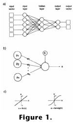
the several ANN learning algorithms available, BP is the most popular (Figure
1A). The BP network consists of an interconnected series of layers, each
containing a number of processing units called `neurons' (Figure
1B). The basic steps in our application of the BP network are: (1) training
of the network on the basis of a number of training sets, and (2) assessment of
the performance of the network by computations of the error rates in the test
sets (details are given below).
Among
the several ANN learning algorithms available, BP is the most popular (Figure
1A). The BP network consists of an interconnected series of layers, each
containing a number of processing units called `neurons' (Figure
1B). The basic steps in our application of the BP network are: (1) training
of the network on the basis of a number of training sets, and (2) assessment of
the performance of the network by computations of the error rates in the test
sets (details are given below).
The main steps in the neural network procedure are
as follows: the input signals (e.g., nannoplankton relative abundances), enter
the network via the input layer; each neuron in the network processes the input
data, with the resulting values steadily seeping through the network layer by
layer, until a result is generated in the output layer. The output of the
network is then compared with the actual output value. This results in an error
value, representing the sum-squared difference between the actual and predicted
input. In order to minimize this error value all the weights at each connection
of the network are gradually adjusted in the direction of the steepest descent
with respect to the error (the steepest-descent algorithm). This process
involves working backwards from the output layer, through the hidden layer, and
back to the input layer, until the specified error limit is reached. Fine-tuning
the weights in this way has the effect of `teaching' the network how to produce
the `desired' output for a particular input. In this way the network `learns'.
The last three steps described above usually have
to be repeated a number of times until the error value is minimized (in the
ideal case this error is zero). These steps may potentially involve many
thousand training passes. This iterative process is the kernel of the back
propagation algorithm. Finally, when the network has converged (meaning, reached
a preset error limit), it will ideally be able to produce the correct output for
each input. Once the network has been trained, it can be used to predict the
output signals used in the training phase from new input signals.
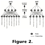 In
the analysis of the dataset from the California Bight, we used five neurons in
the input layer (corresponding to the five species of nannoplankton used as
input variables). In the Mediterranean dataset, we used eight neurons in the
input layer. In both cases, the number of neurons in the output layer is one
(corresponding to the SST and oxygen isotope data to be predicted; Figure
2). The software used was the NeuroGenetic Optimizer (NGO), version 2.6,
from BioComp Systems,
Inc.
In
the analysis of the dataset from the California Bight, we used five neurons in
the input layer (corresponding to the five species of nannoplankton used as
input variables). In the Mediterranean dataset, we used eight neurons in the
input layer. In both cases, the number of neurons in the output layer is one
(corresponding to the SST and oxygen isotope data to be predicted; Figure
2). The software used was the NeuroGenetic Optimizer (NGO), version 2.6,
from BioComp Systems,
Inc.
This program automatically attempts either one or
two hidden layers to find the optimum network. The program also allows the
number of network cycles to be specified prior to the start of the data
processing. Each of these cycles utilizes a different network configuration. The
cycles are divided into populations and generations that can both be varied. In
addition, the program searches the best solution by varying the different number
of neurons in each of the different layers. The NeuroGenetic Optimizer attempts
different types of transfer functions within single neurons (linear, logarithmic
and hyperbolic tangent) when performing genetic searches.