METHODS
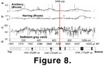 Our data set of digitized laminae thickness, and gray-scale variation, relates directly to annual precipitation (winter terrigenous laminae) and annual productivity (summer diatom laminae). The darker terrigenous laminae, consist of silt, organic debris, and robust diatoms are deposited during the rainy winter months when there is increased runoff. The lighter laminae are comprised primarily of diatoms frustules and are deposited from spring through fall when productivity is enhanced
(Chang et al. 2003;
Figure 8). The relative thickness and color of laminae vary over time in response to changing environmental conditions. Gray-scale analyses of these changes provide an extensive time series that can be used to track this climatic and oceanographic variability
(Figure 7, Figure
8). The abundance of fish scales of Northern Anchovy and Pacific Herring in the core have been used in association with the sedimentological data to compile an additional time-series.
Our data set of digitized laminae thickness, and gray-scale variation, relates directly to annual precipitation (winter terrigenous laminae) and annual productivity (summer diatom laminae). The darker terrigenous laminae, consist of silt, organic debris, and robust diatoms are deposited during the rainy winter months when there is increased runoff. The lighter laminae are comprised primarily of diatoms frustules and are deposited from spring through fall when productivity is enhanced
(Chang et al. 2003;
Figure 8). The relative thickness and color of laminae vary over time in response to changing environmental conditions. Gray-scale analyses of these changes provide an extensive time series that can be used to track this climatic and oceanographic variability
(Figure 7, Figure
8). The abundance of fish scales of Northern Anchovy and Pacific Herring in the core have been used in association with the sedimentological data to compile an additional time-series.
Independent confirmation that the observed laminations represent annual deposition has been provided by detailed
14C and diatom analysis of core TUL99B-03 (Table
1) as well as detailed diatom analysis and
137Cs and 210Pb dating of the 120 cm freeze core (TUL99B-04) collected nearby
(Chang et al.
2003). Physical measurement of annual laminae and accurate
14C ages (Figure 8) indicate that sedimentation rate was nearly constant throughout the studied interval
(Dallimore
2001).
Detailed sedimentological and 14C analysis of seven piston cores collected within adjoining basins of Effingham Inlet as part of a larger study revealed similar stratigraphic successions
(Dallimore
2001), so that the patterns recognized in piston core TUL99B-03 are consistent with actual depositional conditions. The upper 280 cm of the core (which was deposited after ~ 1,800 y BP) was not analyzed here because this portion was very unconsolidated, resulting in poor recovery of sedimentary laminations. Similarly, the lower 150 cm of the core was not analyzed because of loss of record continuity from massive intervals and earthquake-related sedimentation disruptions
(Dallimore
2001).
Mathematical-Statistical Methods
We applied continuous wavelet analysis, spectral analysis, and cross-spectral analysis to our datasets in order to quantify the trends, cyclicity, and bandwidth dependent relations between the different time-series. We used the percentages of taxa present rather than the absolute values in most of the time-series analyses.
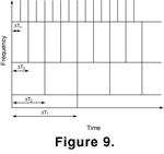 Continuous wavelet transforms are mathematical correlation functions that partition data series into different frequency components as functions of time
(Figure 9). Each component is then studied at a resolution appropriate to its time- or depth scale
(Graps
1995). By examining the entire data set over all frequency bands any cyclic patterns contained in the data series can be identified. This approach is not new.
Fourier (1822) discovered that any function can be closely approximated by a superposition sines and cosines. What is novel about the CWT is the simultaneous function approximation in both time- and frequency- scales, using variable analysis window sizes. Analysis of a signal with a long time (or depth) window permits for high resolution of the frequency content of the data, revealing gross features in the time series. In the case of stratigraphic data, such long windows are needed for low-frequency cycles spanning longer time periods. Analysis of signals with a short time (or depth)l window permits low resolution or shorter duration feature in the frequency pattern. In the context of analyzing stratigraphic data this characteristic permits recognition of high-frequency cycles or abrupt `jumps' (caused by unconformities, sequence boundaries, etc.). CWT is therefore ideal for identifying the patterns typically found in stratigraphic geological data. Wavelet coefficients can also be plotted along a time axis permitting easy recognition of cycles or discontinuities in the data time and frequency scales. Since CWT operates at all scales researchers can "see both the forest and the trees
(Graps
1995)," a characteristic well suited to geological research.
Continuous wavelet transforms are mathematical correlation functions that partition data series into different frequency components as functions of time
(Figure 9). Each component is then studied at a resolution appropriate to its time- or depth scale
(Graps
1995). By examining the entire data set over all frequency bands any cyclic patterns contained in the data series can be identified. This approach is not new.
Fourier (1822) discovered that any function can be closely approximated by a superposition sines and cosines. What is novel about the CWT is the simultaneous function approximation in both time- and frequency- scales, using variable analysis window sizes. Analysis of a signal with a long time (or depth) window permits for high resolution of the frequency content of the data, revealing gross features in the time series. In the case of stratigraphic data, such long windows are needed for low-frequency cycles spanning longer time periods. Analysis of signals with a short time (or depth)l window permits low resolution or shorter duration feature in the frequency pattern. In the context of analyzing stratigraphic data this characteristic permits recognition of high-frequency cycles or abrupt `jumps' (caused by unconformities, sequence boundaries, etc.). CWT is therefore ideal for identifying the patterns typically found in stratigraphic geological data. Wavelet coefficients can also be plotted along a time axis permitting easy recognition of cycles or discontinuities in the data time and frequency scales. Since CWT operates at all scales researchers can "see both the forest and the trees
(Graps
1995)," a characteristic well suited to geological research.
In contrast the sines and cosines that form the basis for Fourier analysis are non-local, and by definition stretch out to infinity. They are useful for examining the frequency content of stationary processes but not useful for approximating the sharp breaks in geological data described above. Wavelet analysis addresses this problem by using approximating functions that are contained in variably scaled finite domains, but has the disadvantage that `edge effects' (suppressed magnitudes for low frequencies) occur for wavelet coefficients at the top and bottom of any analyzed time series. Wavelet analysis
is limited by the Uncertainty Principle whereby higher resolution in time means lower resolution in frequency, and vice versa
(Emery and Thomson
2001).
For a time series, f(t) CWT produces a space of wavelet coefficients
 (a, b), of scale (e.g., wavelength)
a and time (or depth) b:
(a, b), of scale (e.g., wavelength)
a and time (or depth) b:
 .(1)
.(1)
We used the Morlet wavelet (scaled and translated)
 (2)
(2)
with l representative of the scaling ratio of the analyzing window, which is set to
l=10 providing particularly good resolution in periodicity (Rioul and Vetterli 1991;
Grossman and Morlet
1984). Using "zero-padding" on the beginning and ends of the data series reduced edge effects of
W. Data were standardized to a mean = 0, and a fitted linear trend line was removed. The graphic representation in the time-frequency space is a
"scalogram."
Squared Coherency Calculation
To test the confidence of cross-spectral analysis we carried out a squared coherency calculation at the 95% confidence level. Using the approach of
Emery and Thomson
(2001), we divided the fish-scale time-series into successive blocks (roughly 3) with 50% overlap and applied a Kaiser-Bessel weighting to the time series prior to applying the Fast Fourier transform (FFT). For this filter, 50% overlap is sufficient to create individual blocks that are essentially independent time series. In the frequency domain, we used band-averaging of adjacent frequency (f) bands such that
df/f = 0.2 for all frequencies. There are about 6 degrees of freedom (DOFs) per band, except at high frequencies where
df becomes large, and the confidence interval becomes smaller. We applied spectral analysis using FFT and coherence (frequency domain) analysis on the fish-scale data and assumed locally uniform spectral levels for estimation of confidence interval estimates. Squared coherency and 95% confidence level indicate that the slight increase of cross-spectral amplitude at high frequencies in the herring-anchovy time-series observed with spectral analysis is not significant.
Fish Scales
Fish scales were well preserved in these sediments, and abundances were measured as the number of scales/cm3 of sediment
(Table 2). To avoid over-counting of fragmented specimens, only scales with intact focal points were included in the analysis.
