EXAMPLE 1: A 2-D EVOLUTIONARY/DISPERSAL PALAEOBIOGEOGRAPHIC RECONSTRUCTION OF EARLY TRIASSIC AMMONOIDS
Overview of the Geological and Palaeogeographic Context
Early Triassic palaeogeography is relatively simple, largely because continents were joined together in a single block known as
Pangea. Pangea was surrounded by a wide ocean (Panthalassa) and partially bisected by the Tethys Sea
(Elmi and Babin
1996). The Triassic was followed by the largest mass extinction ever at the Permo-Triassic boundary. During this crisis, more than 90% of marine species disappeared
(Raup and Sepkoski
1982). The reef fauna was severely affected and during this period trilobites became extinct
(Erwin 1993,
1994). The Early Triassic appears to have been marked by poorly diversified faunal communities, composed of mobile species and a high percentage of predators
(Erwin 1998,
2001). The
Permo-Triassic crisis is considered to be the Phanerozoic's most drastic reorganisation of ecosystems and animal diversity.
By the Late Permian latitudinal temperature gradients were steep, but, in the late Upper Permian and in the earliest Triassic
(Griesbachian), latitudinal temperature gradients were warmer and weaker from the pole to the equator. This change can be inferred from both the fossil record and climatic simulations
(Hotinski et al. 2001,
Kidder and Worsley
2004). The evolution of the latitudinal temperature gradient during the rest of the Early Triassic
(Dienerian, Smithian, and Spathian) is still poorly understood (Kidder and Worsley
2004). However, the recovery of marine and terrestrial organisms following the crisis was reached by the
Spathian/Anisian boundary (Erwin and Pan
1996), indicating that the latitudinal temperature gradient probably shifted by that time, with colder temperatures at high latitudes.
Ammonoids were the most prominent marine group during the earliest Triassic (Kummel 1973;
Tozer
1973), when they were cosmopolitan with few species. The situation changed through quick diversification and organisation into latitudinal gradients of species richness
(Dagys
1988). The greatest biogeographic differentiation of ammonoid faunas was observed in the Spathian with high endemism in boreal ammonoids
(Dagys
1997). There were no important palaeogeographic events during the Early Triassic, which makes it an appropriate period to study the climatic influence on the biodiversity of ammonoids or other marine organisms possessing at least one planktonic or
pseudo-planktonic living stage. We used a numerical model of the Early Triassic
palaeogeography, to simulate the redistribution of biodiversity and the evolution of planktonic or
pseudo-planktonic organisms, in response to parameters such as SST, SSC, and speciation and extinction rates.
Algorithm
The probabilistic model presented below uses two physical environmental factors (SST and
SSC) to control geographic displacements, speciation events, and extinction of planktonic species
(Brayard
2002). We used an algorithm based on the idea of cellular automata. These automata are divided in modules interacting with each other via action or reaction loops. Depending on local conditions, numerical objects (e.g., cells, sand particles) can interact and self-organize, creating spatial and temporal patterns
(Wootton
2001).
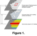 The program was designed in three parts (Figure
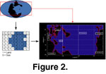
1). The main module built the Early Triassic palaeogeography from a digitized version of a published reconstruction
(Smith et al. 1994, from 60° North and 60° South and from 180° West to 180° East,
Figure 2). The geographic space is represented as an X * Y matrix corresponding to the longitudinal (X) and latitudinal (Y) subdivisions in which each grid-cell represents a quadrate of 360/X° by 120/Y°. Land is coded as 1 and sea as 0. The system also handled the biogeographic distribution of n simulated species whose presence (coded as number 1) or absence (coded as number 0) are saved in a matrix with dimensions X * Y * n, where n is the number of species.
The program was designed in three parts (Figure
1). The main module built the Early Triassic palaeogeography from a digitized version of a published reconstruction
(Smith et al. 1994, from 60° North and 60° South and from 180° West to 180° East,
Figure 2). The geographic space is represented as an X * Y matrix corresponding to the longitudinal (X) and latitudinal (Y) subdivisions in which each grid-cell represents a quadrate of 360/X° by 120/Y°. Land is coded as 1 and sea as 0. The system also handled the biogeographic distribution of n simulated species whose presence (coded as number 1) or absence (coded as number 0) are saved in a matrix with dimensions X * Y * n, where n is the number of species.
 The second module applied a latitudinal gradient of SST to the X * Y * n biogeographic matrix, which constrains geographic displacements, speciation events, and local extinctions for each simulated species based on a fixed or random thermal range for that species. Because the shape, intensity, and evolution of the SST gradient through the Early Triassic are actually unknown, we constructed a number of hypothetical SST gradients using the present-day Pacific gradient as a starting point (data from the
National Oceanic and Atmospheric Administration). Even if the Panthalassic Ocean was significantly wider than the modern Pacific, the choice of the Pacific SST gradient as a model is justified by the global geographic similarity between the two.
The second module applied a latitudinal gradient of SST to the X * Y * n biogeographic matrix, which constrains geographic displacements, speciation events, and local extinctions for each simulated species based on a fixed or random thermal range for that species. Because the shape, intensity, and evolution of the SST gradient through the Early Triassic are actually unknown, we constructed a number of hypothetical SST gradients using the present-day Pacific gradient as a starting point (data from the
National Oceanic and Atmospheric Administration). Even if the Panthalassic Ocean was significantly wider than the modern Pacific, the choice of the Pacific SST gradient as a model is justified by the global geographic similarity between the two.
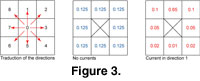 The third module managed the distribution, direction, and intensity of oceanic currents. The module is activated every time a species displacement on the biogeographic grid is called for. We also derived the Early Triassic current configuration from the present-day Pacific as represented in the current data published by
Pickard and Emery
(1990). The matrix of currents was constructed by choosing a single direction of current (among eight possible directions) for each cell. Each direction was coded by a number from one to eight. Zero is equivalent to the lack of a current and therefore equal probability of displacement in any directions
(Figure 3). Current intensity was represented using discrete probabilities of displacements – the higher the probability in one direction, the higher the strength of the current
(Figure 3). Use of continuous probabilities (e.g., calculated from equations of diffusion and advection) would make the displacements more realistic; nevertheless, it would involve serious complications in computation without affecting the broader-scale simulation results.
The third module managed the distribution, direction, and intensity of oceanic currents. The module is activated every time a species displacement on the biogeographic grid is called for. We also derived the Early Triassic current configuration from the present-day Pacific as represented in the current data published by
Pickard and Emery
(1990). The matrix of currents was constructed by choosing a single direction of current (among eight possible directions) for each cell. Each direction was coded by a number from one to eight. Zero is equivalent to the lack of a current and therefore equal probability of displacement in any directions
(Figure 3). Current intensity was represented using discrete probabilities of displacements – the higher the probability in one direction, the higher the strength of the current
(Figure 3). Use of continuous probabilities (e.g., calculated from equations of diffusion and advection) would make the displacements more realistic; nevertheless, it would involve serious complications in computation without affecting the broader-scale simulation results.
 The algorithm of the program can be divided in five successive steps where our parameters are successively tested:
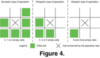
- Speciation: Given a fixed probability of speciation, a new species can be created in a cell occupied by its "parent-species."
 Three types of speciation events were distinguished: sympatric,
parapatric, and allopatric, each with its own probability of occurrence. The type of speciation depended on the number and location of adjacent filled cells
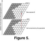
(Figure 4). Speciation probability and number of surrounding filled cells were inversely correlated. A species was added
(cladogenesis) to the biogeographic matrix in the form of a supplementary layer by extending the n-dimension
(Figure 5).
Three types of speciation events were distinguished: sympatric,
parapatric, and allopatric, each with its own probability of occurrence. The type of speciation depended on the number and location of adjacent filled cells
(Figure 4). Speciation probability and number of surrounding filled cells were inversely correlated. A species was added
(cladogenesis) to the biogeographic matrix in the form of a supplementary layer by extending the n-dimension
(Figure 5).
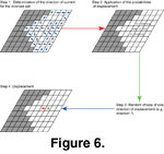 Displacement: A species occupying a cell can move to surrounding cells only if those cells are not already filled with the same species, and only if displacements in that direction are allowed by the superimposed oceanic currents. The module managed displacements in four successive steps in which first current direction, then intensity, then species displacement direction, and finally displacement success were determined
(Figure 6).
Displacement: A species occupying a cell can move to surrounding cells only if those cells are not already filled with the same species, and only if displacements in that direction are allowed by the superimposed oceanic currents. The module managed displacements in four successive steps in which first current direction, then intensity, then species displacement direction, and finally displacement success were determined
(Figure 6).
- Extinction: Two cases were distinguished: "local" and "complete" extinction, each having its own probability of occurrence. A species extinction in a filled cell ("local" extinction) did not affect the neighbouring cell filled with this species. In the case of a "complete" extinction, all cells filled with the same species are simultaneously emptied.
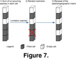 Diversity check: The program checked for cells whose diversity threshold has been reached to avoid an ecologically unrealistic accumulation of species
(Figure 7).
Diversity check: The program checked for cells whose diversity threshold has been reached to avoid an ecologically unrealistic accumulation of species
(Figure 7).
- Species richness monitoring: Finally, the program calculated the species richness for each cell as the sum of co-occurring species.
Even if these five steps are successively executed for each cell and time iteration, speciation, extinction, and displacement events do not necessarily occur. As a result, the evolutionary rate of each cell is independent from cell to cell.
Results
Running our model for several hundred iterations (depending on the SST gradient and the selected speciation and extinction rates) allows us to construct theoretical patterns of species richness distribution under SST and SSC constraints. These theoretical patterns can be compared to the real ones observed in Early Triassic
ammonoids.
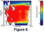 Simulation Running without Currents and with a Weak SST Gradient. As a benchmark, we ran a simulation with no SSC and only a weak SST gradient, implying a weak or nil latitudinal and/or longitudinal bias in the geographic distribution of the simulated species. The results represent a random and thus statistically homogeneous distribution of the simulated species
(Figure 8): simulated species are logically not organized along a diversity gradient. This example may correspond to the wide palaeogeographic distribution of the first earliest Triassic invertebrate marine species (like the two surviving ammonoid genera
Otoceras or Ophiceras, Lingula for brachiopods or Claria for bivalves;
Kummel 1973,
Erwin and Pan
1996). This null model suggests that the SST gradient strongly influences the emergence and the general structure of a latitudinal gradient of species richness
(LGSR).
Simulation Running without Currents and with a Weak SST Gradient. As a benchmark, we ran a simulation with no SSC and only a weak SST gradient, implying a weak or nil latitudinal and/or longitudinal bias in the geographic distribution of the simulated species. The results represent a random and thus statistically homogeneous distribution of the simulated species
(Figure 8): simulated species are logically not organized along a diversity gradient. This example may correspond to the wide palaeogeographic distribution of the first earliest Triassic invertebrate marine species (like the two surviving ammonoid genera
Otoceras or Ophiceras, Lingula for brachiopods or Claria for bivalves;
Kummel 1973,
Erwin and Pan
1996). This null model suggests that the SST gradient strongly influences the emergence and the general structure of a latitudinal gradient of species richness
(LGSR).
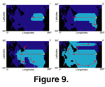 Impacts of Currents on the Simulation. In order to visualize the impact of currents, we can apply them fully, partially, or not at all. If we impose no diffusion and only transport in the direction of the current, the species is destined to stay in the oceanic gyres for many iterations, but if we allow both diffusion and transport in the direction of the current, species are distributed along the principal currents, as well as in intermediate zones
(Figure 9.1-4). Our simulations indicate that currents have a strong influence only over the timing (especially on the dispersal throughout the
Panthalassa) and local patterns of dispersion of the simulated species. They have no influence on the shape and magnitude of the simulated LGSR on a global scale. If we remove currents from the simulation, the general shape and magnitude of the LGSR is conserved. Mixed water assemblages driven by currents do not seem to be the preponderant factor for explaining patterns of low species diversity in some convergence zones (e.g., equatorial, contra
Casey 1989;
Rutherford et al. 1999;
Kiessling
2002).
Impacts of Currents on the Simulation. In order to visualize the impact of currents, we can apply them fully, partially, or not at all. If we impose no diffusion and only transport in the direction of the current, the species is destined to stay in the oceanic gyres for many iterations, but if we allow both diffusion and transport in the direction of the current, species are distributed along the principal currents, as well as in intermediate zones
(Figure 9.1-4). Our simulations indicate that currents have a strong influence only over the timing (especially on the dispersal throughout the
Panthalassa) and local patterns of dispersion of the simulated species. They have no influence on the shape and magnitude of the simulated LGSR on a global scale. If we remove currents from the simulation, the general shape and magnitude of the LGSR is conserved. Mixed water assemblages driven by currents do not seem to be the preponderant factor for explaining patterns of low species diversity in some convergence zones (e.g., equatorial, contra
Casey 1989;
Rutherford et al. 1999;
Kiessling
2002).
Simulations with the Present-Day SST Gradient. If we apply the present-day SST gradient to the model, we might expect a LGSR similar to the classical view of species richness increasing monotonically and regularly from the poles to the equator. This pattern has been recognized in terrestrial and marine environments and for faunas and floras from all geological time periods
(Stehli et al. 1969;
Schopf 1970;
Rex et al. 1993;
Gaston 2000;
Crame 2002; see also
Rhodes 1992 for a review of hypotheses about the formation of latitudinal gradients in species richness).
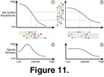
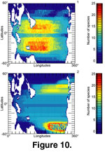 However, our results suggest a quite different pattern with a slight decrease in species richness near the equator
(Figure 10.1). In fact, most of the simulations found maximal species richnesses close to the Tropics of Cancer and Capricorn. This pattern results from the geometric overlap of the species distributions as influenced by the shape and intensity of the SST gradient
(Figure 11). This by-product of superimposed thermal ranges has been described in the modern setting as the "mid-domain effect"
(Colwell and Hurtt 1994,
Colwell and Lees, 2000,
Colwell et al.
2004). This principle suggests that observed LGSR may simply be the result of chance. In situations with two fixed boundaries, randomly distributed ranges never generate a uniform spatial distribution but always give rise to a peak or a plateau of species richness. In the absence of any environmental or historical gradients, the formation of an LGSR may be solely the consequence of the spatial distribution of the thermal ranges of species as controlled by the SST gradient.
However, our results suggest a quite different pattern with a slight decrease in species richness near the equator
(Figure 10.1). In fact, most of the simulations found maximal species richnesses close to the Tropics of Cancer and Capricorn. This pattern results from the geometric overlap of the species distributions as influenced by the shape and intensity of the SST gradient
(Figure 11). This by-product of superimposed thermal ranges has been described in the modern setting as the "mid-domain effect"
(Colwell and Hurtt 1994,
Colwell and Lees, 2000,
Colwell et al.
2004). This principle suggests that observed LGSR may simply be the result of chance. In situations with two fixed boundaries, randomly distributed ranges never generate a uniform spatial distribution but always give rise to a peak or a plateau of species richness. In the absence of any environmental or historical gradients, the formation of an LGSR may be solely the consequence of the spatial distribution of the thermal ranges of species as controlled by the SST gradient.
 If we change the SST gradient, the LGSR also changes
(Figure 8). If a change takes place in the thermal ranges of species or in the position of the ancestral species, the LGSR is immediately affected (example in
Figure 10.2).
If we change the SST gradient, the LGSR also changes
(Figure 8). If a change takes place in the thermal ranges of species or in the position of the ancestral species, the LGSR is immediately affected (example in
Figure 10.2).
Our simulation thus indicates that the formation of a gradient of taxonomic richness for marine organisms with at least one planktonic or
pseudo-planktonic stage can be partially, if not completely due to: 1) the superimposition of species thermal ranges according to the geometry of the SST gradient; 2) the evolutionary history of the taxa (latitudinal position of the lineage origination); and 3) the characteristic parameters of individual species affecting the local species distribution.
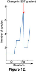 Simulation of a Changing SST Gradient Applied to the Early Triassic. The SST gradient can be changed at any given iteration of a simulation. When a simulation starts with the present-day SST gradient and then a weak SST gradient is applied, the species distribution becomes homogenized and cosmopolitan. Species whose thermal range excludes them from the coldest temperatures disappear. When we change the SST gradient to be warmer and weaker, only tropical species survive after which they colonize higher latitudes. However, with a colder, weaker SST gradient, only high latitudes species survive and progressively invade low latitudes. If we proceed in reverse, setting a weak SST gradient at the start and abruptly changing it to a very steep one, we obtain a drop in the total species richness
(Figure 12).
Simulation of a Changing SST Gradient Applied to the Early Triassic. The SST gradient can be changed at any given iteration of a simulation. When a simulation starts with the present-day SST gradient and then a weak SST gradient is applied, the species distribution becomes homogenized and cosmopolitan. Species whose thermal range excludes them from the coldest temperatures disappear. When we change the SST gradient to be warmer and weaker, only tropical species survive after which they colonize higher latitudes. However, with a colder, weaker SST gradient, only high latitudes species survive and progressively invade low latitudes. If we proceed in reverse, setting a weak SST gradient at the start and abruptly changing it to a very steep one, we obtain a drop in the total species richness
(Figure 12).
All thermal variations yield disruptions in species richness. On a global scale, this type of simulation can easily represent climatic changes in time and space and their consequences on the distribution of species on Earth. Changes of the SST gradient during the simulation evoke changes that reproduce observed diversity curves.
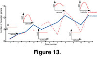 For example, in
Figure 13 we identified a sequence of changes to the SST gradient that can be hypothesized to have occurred during the Early Triassic. The SST parameters of the program were iteratively constrained to produce a species richness curve that maximally corresponds to the real diversity curve. The beginning of the simulation corresponds to the weak and warm pole-to-equator SST gradient of the
Permo-Triassic boundary. Principal observations are: 1) a lowering of the SST gradient corresponds to a decreasing of endemism; 2) a steepening of the SST gradient leads to an increase of latitudinally restricted
taxa.
For example, in
Figure 13 we identified a sequence of changes to the SST gradient that can be hypothesized to have occurred during the Early Triassic. The SST parameters of the program were iteratively constrained to produce a species richness curve that maximally corresponds to the real diversity curve. The beginning of the simulation corresponds to the weak and warm pole-to-equator SST gradient of the
Permo-Triassic boundary. Principal observations are: 1) a lowering of the SST gradient corresponds to a decreasing of endemism; 2) a steepening of the SST gradient leads to an increase of latitudinally restricted
taxa.
The recovery of ammonoids after the Permo-Triassic extinction was not a continuous increase in species richness
(Figure 13) or of the steepness of the
LGSR, but was a sequence of increases and decreases. These fluctuations also differed
latitudinally. In spite of their geographic complexity, our simulation indicates that the fluctuations of species richness can easily be modelled with simple changes in the SST gradient, which strongly suggests that such SST gradient directly influences the marine species richness and its distribution on Earth.
It appears that the formation of global-scale marine LGSR may be due to the shape and magnitude of the SST gradient, and to the location of the ancestral species. Even if it seems problematic to invoke only a single biotic (e.g., physiologic) and/or abiotic (physical environment) factor, the origin of the latitudinal species richness gradient can be the simple geometric by-product of the geographic overlap of thermally constrained species ranges. Through our model, IDL improved the visual understanding of the consequences of a changing climate on the distribution of species. IDL is completely adapted to run and visualize biogeographic models with an evolutionary time dimension.
