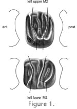
METHODS

The three mentioned groups of Bransatoglirinae, and the Dryomyinae, Glamyinae, Gliravinae, Glirinae, and Myomiminae form the eight groups for which concavity will be compared.

We drew over 500 profiles in anterior and posterior view of lower and upper M1 and M2 of the available specimens of M₁, M₂, M¹, and M² with a camera lucida mounted on a Wild M8 or Wild M5 binocular microscope, normally at 50x magnification, but at 25x for the largest specimens.

Instead of using lengthy terms like 'anterior profile of M₁', 'posterior profile of M²' we will use descriptive names for the eight profile classes: m1inf_ant, m1inf_post, m2inf_ant, m2inf_post, m1sup_ant, m1sup_post, m2sup_ant, and m2sup_post.

The anterior profile of the upper molars was drawn over the paracone and the anterior corner of the protocone, which are the most characteristic points of the profile in anterior view. Similarly, the posterior profile was drawn over the metacone and the posterior corner of the protocone. In the lower molars the metaconid and protoconid define the anterior view, and the entoconid and hypoconid the posterior view. In other words the curves do not represent the anterior or posterior border, respectively, of the tooth. The shape and height of anteroloph(id) and posteroloph(id) may vary considerably within a sample, and should not be used to define the concavity of a specimen. In Figure 1 the location of the profiles in the occlusal surface is indicated. It also makes clear why the anteroloph is not suitable to define concavity.

Most of the computational work might have been performed using commercial computer programs, but in view of the large amount of data to be processed we decided to write a set of programs in Visual Basic. One of these programs allows the tracing of bitmaps (raster images). It converts the bitmaps into vector images by creating lines that connect the dots of a bitmap, and then it converts the vectors into a polygon. Once the polygon is created, a second program serves to calculate a standard set of parameters through the methods of analytic geometry, and a third one performs many comparisons of these parameters.

The drawings, as well as the published figures, were scanned, and the resulting bitmaps were oriented so that the occlusal side faced down. The figure was inverted if necessary so that the protocone/protoconid side faced left. This standardized orientation facilitates automatic computation. Then the bitmaps were vectorized (converted into polygons), and the polygons were exported to files in Hewlett Packard Graphics Language (HPGL) format. The number of vertices (v) in the occlusal concavity part of the polygon was chosen to lie between 15 and 20.

After this, the profiles were analyzed, parameters were calculated for each one, text labels were associated with the image, and the results were written to a text file.

Results for each of the eight profile classes (two profiles for each first and second molar, upper and lower) were compiled into a single text file that served as input to the next program that performed the comparisons of the parameters within profile classes and between profile classes, and which also produced graphic representations of the results.

The parameters are indicated in Figure 2: w is the maximum width of the molar as seen in the profile, x and y are the limits of the occlusal concavity: the top of the protocone, paracone, metacone, protoconid, metaconid, hypoconid, or entoconid, depending on the element in question, and the direction of the view. The letter b (base) designates the distance between x and y, h (height) is the maximum depth of the concavity, and S is the surface of the area enclosed by b and the occlusal profile. The lines b1 and b2 are the portions of b defined by its intersection with h. The drawings have been rescaled, so that w = 10 in all cases; a test has shown that rescaling to b makes no difference in the results.

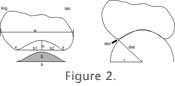
The occlusal concavity of the profile of Figure 2 is a polygon, consisting of between 15 and 20 vertices connected by straight lines. To automate the process of finding the circle that best fits the concavity, circles were first constructed through all combinations of three vertices of the occlusal concavity, and the radius and center of each circle were calculated. Those circles with a center higher than the occlusal profile were discarded, because they correspond to convex parts of the profile; the distribution of the radii of all remaining circles was calculated, and the circles with extremely high or low values were discarded, too. Discarding 5% of the circles on each side of the distribution turned out to be a suitable procedure. Then a circle was drawn with its center at the mean of all circle centers, and a radius r corresponding to the mean of the radii. The radius of this circle was considered to be a first approximation of the circle that best fits the original curve. In the next step, the center of this circle was connected to all vertices, and the sum of the absolute values of the deviations d-r was calculated as dev=Σ |dist-r|, where dist is the distance from the circle center to the vertex. Then the circle was shrunk and wobbled through several thousand iterations to find the radius and the position of the circle that gave the lowest value for dev, and the radius r of that circle was then used as a measure of concavity. In the tables where dev is listed, it is divided by the number of vertices v to standardize for v.

Several commercial computer programs permit drawing circles on bitmaps, and changing the position and radius of these circles. Our program makes this process much easier and maximizes precision, but results obtained through a program like Corel Draw are perfectly compatible, as we have tested by manually creating the circles and comparing them with the automatically obtained results. The difference of the radius of the programmatically calculated circle, and the one constructed manually in our tests, did not exceed 5%.