Methods

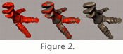
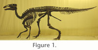Following on from previous work, we used the GaitSym simulation system based on the Open Dynamics Engine (ODE) (Sellers and Manning 2007). To produce the musculoskeletal model, a mounted skeleton of a juvenile Edmontosaurus annectens (BHI 126950) was photographed (Figure 1) and measured, and selected elements were laser scanned using a Polhemus FastSCAN system (complete hindlimb and forelimb, limb girdles, skull and representative vertebrae and ribs). This system allows detailed scanning using a short-range laser scanner with the advantage that both the scanning head and the object being scanned can be freely moved, which is especially useful when scanning complex objects such as vertebrae and skulls. 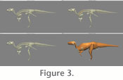The raw scan files were exported from the proprietary FastSCAN software in .obj format and imported into Maya where bone outlines were fitted to the scans (Figure 2). This process allows correcting for distortion, and the idealised geometries produced have a much lower polygon count, which allows them to be used efficiently for later visualisation, animation and modelling. The individual, re-inflated bones are then articulated within Dinomorph where joint centres and ranges of motion are defined, and the rearticulated model is re-exported to Maya to allow the construction of the body segment geometry and to define origin and insertion points of muscles (Figure 3) for import into GaitSym. A detailed description of the recommended workflow for creating models can be found in the GaitSym user manual available at Animal Simulation Laboratory.

With current technology it is relatively easy to simulate the contraction of a large number of muscles, but treating each muscle as a separate entity (or even functionally subdividing muscles) produces extremely complex gait controllers, and our current system cannot find suitable contraction patterns in a reasonable length of time. The complexity can be reduced considerably by grouping functionally equivalent muscles. The hindlimb musculature was taken from Dilkes (2000) and the forelimb musculature from Schachner (2005) and composite muscle groupings produced depending on action (groupings named after Carrano and Hutchinson 2002). Deciding the muscle mass to assign is problematic, but for consistency with previous work we chose a figure of 30% of body mass for extensor musculature (Hutchinson 2004a; Hutchinson 2004b; Sellers and Manning 2007) and 20% of body mass for flexor muscle mass (Sellers and Manning 2007). However, we note that these values are likely to be towards the upper end of plausible muscle mass estimates (Grand 1977; Hutchinson and Garcia 2002). Dividing this total muscle mass among even a simplified range of muscles is similarly difficult and so the pragmatic solution of dividing equally among the joints of each leg was chosen and in the case of the quadrupedal simulation an arbitrary division was made such that 30% of the muscle mass was in the forelimb and 70% in the hindlimb reflecting the covariation in limb geometry for Edmontosaurus. Even then there are muscle groups that have an action over more than one joint, and in these cases they receive a mass proportion from each joint. The fibre lengths and tendon lengths were calculated by measuring the minimum and maximum length of each composite muscle obtained by moving the joints through their full ranges of motion and using the length change for the fibre length and the mean overall length minus the fibre length as the tendon length. This is likely to be a fairly optimal length for any muscle since vertebrate muscles are typically able to generate force from approximately 60% to 160% of their resting length (McGinnis 1999). Using length change through joint range of motion as a way of defining fibre length also eliminates any uncertainty over moment arm since the leverage gain of a larger moment arm is exactly balanced by the force production loss for a given mass of muscle. Physiological cross section area is calculated from fibre length and muscle volume assuming a muscle density of 1056 kg m^-3 (Winter 1990). All muscle information is shown in Table 1. Segmental mass properties were generated automatically from the body outlines using a body density of 1000 kg m^-3 (Henderson 1999). The total volume was also used to estimate a total body mass of 715.3 kg. Limited experimentation was performed using alternative densities and including air sacs (Alexander 1989) but the differences found were small and have therefore been ignored since the uncertainty in the body outlines is likely to be a much larger source of error. The models are fully three-dimensional but all joints are hinge joints allowing only parasagittal rotation to keep the model at manageable levels of complexity. The full specification of each model as a human readable XML file is available for download the Animal Simulation Laboratory website. The version for galloping is included in the Appendix.

The muscles were activated by a 5-phase pattern. This was applied to each muscle for a fixed duration, and then the left and right hand side patterns were swapped and reapplied. A complete gait cycle thus consisted of 5 distinct activation patterns for 32 muscles plus the cycle duration: a total of 161 parameters. The musculoskeletal model as placed in a stationary, upright pose with the forelimb tightly flexed in the bipedal models but extended in the quadrupedal model, and this was used as the starting condition for the genetic algorithm optimisation process. This process has been described in detail elsewhere (Sellers et al. 2003; Sellers and Crompton 2004; Sellers et al. 2005) but in brief it proceeds by cycling through a testing phase, a selection phase and a reproduction phase. We start with 1000 random activation patterns, and these patterns are tested by applying these to the model and running the simulation to see how far that activation pattern can drive the model forward in 5 seconds of simulated time. This test evaluates the fitness of these patterns with the fittest being able to drive the model a little further forward than the others. This procedures is then followed by a selection phase where 'roulette wheel' algorithm (Davis 1991) is used to select which of the original 1000 patterns is used as a model, which means that the best of the previous patterns are more likely to contribute to subsequent patterns, and the best 100 patterns are retained for subsequent generations in any case. In this algorithm the roulette wheel is biased so the likelihood of random selection is proportional to the forward distance achieved by the pattern.

In the reproduction phase another 1000 patterns are then created using the selected patterns as models and then adding a small amount of random variation or by merging parts of two patterns (this alteration process is sometimes referred to as mutation). The new patterns are then entered into the cyclic process again where they are tested, selected and reproduced as before. There is a reasonable likelihood that one of the new patterns will work better than the ones in the previous generation. This process is repeated 1000 times or until no improvement has been detected for 100 repeats. At the end of this process, from a standing start, some form of forward locomotion will have been generated. Rather than begin again from a standing start with a new random set of patterns, a new set of initial conditions are generated from the simulation by taking a snapshot of the model state after one gait cycle. This state is now a dynamic starting condition with velocities as well as positions for all the segments and enables us to bootstrap the simulation process since we are aiming to simulate steady state locomotion rather than acceleration. We also use the previous best set of patterns as the starting set of patterns since these are likely to be good patterns for the new starting conditions. The whole process (1000 batches of new patterns) is then repeated, and this process of restarting from a new set of initial conditions generated from a previous run is repeated 20 times. This simulation has potentially been run 20 × 1000 × 1000 times although usually because of the termination after no improvement rule it is usually about half this value i.e., 10,000,000 repeats. In this particular project this process was performed for both the bipedal model and for the quadrupedal model, and each model was repeated 10 times. Given that the simulator runs in roughly half real time, over 10,000 days of CPU time is represented. Fortunately the system is able to run on multiple computers simultaneously so this amount of computing power is relatively manageable.

After optimisation, the best runs are chosen from each of the 20 top level repeats, and these are visualised and the gait classified. The gaits are generated randomly, and the same selective effort has been put into each case so these should be an unbiased estimate of the locomotor capabilities of the quadrupedal and bipedal forms. The random noise added is normally distributed so given long enough each run can theoretically explore the whole of the gait search space. Experience has shown that with this amount of computational effort it will tend to stabilise around a local rather than a global optima that allows it to find a range of sub-optimal gaits but to produce high quality gait within these sub-optima. However, it was hoped that with 10 repeats it would be possible to detect patterns of preferred gait: gaits that either occupy a large proportion of the search space or that produce consistently higher speed than other gaits. The gait types produced were visually identified. Selected gaits were also further optimised using a lower total run time (3 seconds) to see whether the requirements of stability were hampering their maximum running speed.